

2. Running TDR#
This notebook uses the production functions in samueleronchini/gw_tdr. It runs the pipeline on public GWOSC strain around GRB 200228A (Fermi trigger bn200228291), the O3 GRB identified in the paper as having the largest \(D_{90}^{\rm TDR}\) and used for its TDR sky-map example. It uses the event’s Fermi/GBM HEALPix localization, then examines detector status, PSDs, antenna response, efficiency curves, TDR map, and result tables.
The trigger time (2020-02-28 06:58:33 UTC) and sky map are from the Fermi/GBM localization circular for GRB 200228A. The map is downloaded from the official HEASARC archive. As in the paper, the TDR is evaluated for assumed representative BNS/NSBH systems.
Requirements: Python 3.11, an editable local installation of gw_tdr and its PyCBC/LALSuite/GWpy dependencies, and network access to GWOSC. The first full run downloads strain and can take several minutes. Outputs and the strain cache are written outside this tutorial tree under ~/.cache/gw_tdr_tutorial/.
2.0 Setup#
Place this notebook after Samuele’s priors notebook in acme_tutorials/tdr/.
Reuse its working TDR environment, or install one in a terminal:
conda create -n gw-tdr python=3.11 pip -y
conda activate gw-tdr
git clone https://github.com/samueleronchini/gw_tdr.git
git clone https://github.com/samueleronchini/acme_tutorials.git
python -m pip install -e ./gw_tdr jupyterlab ipykernel pymupdf tqdm
python -m ipykernel install --user --name gw-tdr --display-name "Python 3.11 (gw_tdr)"
Skip clones you already have. TDR also requires wget or curl.
Launch Jupyter from the notebook directory so all generated folders stay alongside it:
cd acme_tutorials/tdr
OMP_NUM_THREADS=1 MKL_NUM_THREADS=1 OPENBLAS_NUM_THREADS=1 jupyter lab
Select the TDR kernel. pymupdf previews the saved PDF; tqdm displays download progress.
# to be used on sciserver
import os, sys
bindir = os.path.dirname(sys.executable)
if bindir not in os.environ["PATH"].split(os.pathsep):
    os.environ["PATH"] = bindir + os.pathsep + os.environ["PATH"]
2.1 Install and orient yourself in the production code#
This notebook requires Python >=3.11 and both the gwosc dependency and the local gw_tdr source package in the same kernel environment. In VS Code, choose the Python 3.11 TDR environment from the notebook kernel picker, then restart the kernel and rerun from the first cell. In a terminal configured for that exact environment, install the local repository with python -m pip install -e /path/to/gw_tdr (replace the path with your clone location); register the environment with python -m pip install ipykernel and python -m ipykernel install --user --name gw-tdr --display-name "Python 3.11 (gw_tdr)" if it is not already listed. The import-check cell reports the current interpreter and identifies whether gwosc or targ_ac_git is missing. The pipeline also uses PyCBC command-line tools; before running, the notebook checks that pycbc_create_injections and pycbc_optimal_snr are available from this environment and adds its scripts directory to the subprocess PATH.
Analysis step |
Production function(s) |
|---|---|
Select observing-run configuration and read GWOSC strain |
|
Estimate and validate PSDs; report usable IFOs |
|
Create reference injections and compute optimal SNR |
|
Apply sky/orientation response and calculate detection fractions / D90 |
|
Draw sky samples and plot the TDR map |
|
The public pipeline evaluates a fixed grid of BNS and NSBH masses (and EOS choices for NSBH). Its inclination prior is isotropic in solid angle, truncated to an interval. It accepts a fixed sky position or a HEALPix sky map; arbitrary joint mass–inclination–sky posterior samples are an exercise at the end, not an existing CLI feature.
# Load plotting/data tools and the production TDR/PyCBC interfaces.
import importlib.util
import json
import os
import shutil
import subprocess
import sys
import sysconfig
import tempfile
from pathlib import Path

import matplotlib.pyplot as plt
import numpy as np
import pandas as pd
from IPython.display import FileLink, Image, display
from pycbc.detector import Detector

# Fail early with an actionable message if this kernel cannot run the real pipeline.
missing_modules = [name for name in ("gwosc", "targ_ac_git") if importlib.util.find_spec(name) is None]
if sys.version_info < (3, 11) or missing_modules:
    raise RuntimeError(
        "This notebook needs Python >=3.11 with the TDR dependencies and local editable installation. "
        f"Current kernel: {sys.executable} (Python {sys.version.split()[0]}). "
        f"Missing modules: {missing_modules}. Install the local gw_tdr checkout into this kernel using "
        "python -m pip install -e /path/to/gw_tdr, then restart the kernel. See §2.1."
    )

from astropy.time import Time
from targ_ac_git import aux_snr_mf as tdr_aux
from targ_ac_git.pipeline_utils_snr_mf import PSDWrapper
from targ_ac_git.targ_range_snr_mf import (
    CHIRP_MASSES,
    choose_localization_samples,
)
from targ_ac_git.gwosc_utils_snr_mf import _get_run_config

# Render production PDF plots inline while retaining a clickable fallback.
def show_pdf(path):
    path = Path(path)
    if not path.is_file():
        raise FileNotFoundError(path)
    renderer = shutil.which("pdftoppm")
    if renderer is None:
        print(f"Inline PDF preview unavailable; open the plot file: {path}")
        display(FileLink(str(path)))
        return

    with tempfile.TemporaryDirectory() as temp_dir:
        image_prefix = Path(temp_dir) / path.stem
        subprocess.run(
            [renderer, "-f", "1", "-singlefile", "-png", "-r", "120", str(path), str(image_prefix)],
            check=True,
            capture_output=True,
            text=True,
        )
        display(Image(filename=f"{image_prefix}.png"))

print("Python:", sys.version.split()[0])
print("Interpreter:", sys.executable)
print("TDR source:", __import__("targ_ac_git").__file__)
/opt/anaconda3/envs/TDR_grb/lib/python3.11/importlib/__init__.py:126: UserWarning: Wswiglal-redir-stdio:

SWIGLAL standard output/error redirection is enabled in IPython.
This may lead to performance penalties. To disable locally, use:

with lal.no_swig_redirect_standard_output_error():
    ...

To disable globally, use:

lal.swig_redirect_standard_output_error(False)

Note however that this will likely lead to error messages from
LAL functions being either misdirected or lost when called from
Jupyter notebooks.

To suppress this warning, use:

import warnings
warnings.filterwarnings("ignore", "Wswiglal-redir-stdio")
import lal

  return _bootstrap._gcd_import(name[level:], package, level)
PyCBC.libutils: pkg-config call failed, setting NO_PKGCONFIG=1
/opt/anaconda3/envs/TDR_grb/lib/python3.11/site-packages/tqdm/auto.py:21: TqdmWarning: IProgress not found. Please update jupyter and ipywidgets. See https://ipywidgets.readthedocs.io/en/stable/user_install.html
  from .autonotebook import tqdm as notebook_tqdm
Python: 3.11.15
Interpreter: /opt/anaconda3/envs/TDR_grb/bin/python
TDR source: /Users/samueleronchini/Desktop/tdr_time/gw_tdr/targ_ac_git/__init__.py
2.2 Select a GRB and run TDR#
The Fermi/GBM Final Real-time Localization circular reports GRB 200228A (bn200228291) at 2020-02-28 06:58:33 UTC (GCN 27247). This lies in LVK O3b. We pass the corresponding HEALPix probability map directly to the TDR command. TDR selects the O3b detector configuration and fetches the configured 256 s public strain interval centered on the GRB time. Set IOTA_MIN_DEG and IOTA_MAX_DEG to the single inclination interval you want before running the pipeline. Set RUN_PIPELINE = False only when reusing a completed output directory for the same trigger, sky map, and analysis settings.
# Configure the trigger, data products, SNR threshold, and the single main-run inclination prior.
EVENT = "GRB200228A"
TRIGGER_ID = "bn200228291"
T0_UTC = "2020-02-28T06:58:33"
T0 = Time(T0_UTC, format="isot", scale="utc").gps
SNR_THRESHOLD = 8.5
SNR_STATISTIC = "mf"  # matched-filter-like convention used by the TDR CLI
OUTPUT_ROOT = Path(os.environ.get("TDR_TUTORIAL_OUTPUT", Path.home() / ".cache" / "gw_tdr_tutorial" / EVENT)).expanduser()
RUN_DIR = OUTPUT_ROOT / "scan_t0p0000"
SKYMAP_URL = "https://heasarc.gsfc.nasa.gov/FTP/fermi/data/gbm/triggers/2020/bn200228291/quicklook/glg_healpix_all_bn200228291.fit"
SKYMAP_FILE = OUTPUT_ROOT / "glg_healpix_all_bn200228291.fit"
OUTPUT_ROOT.mkdir(parents=True, exist_ok=True)

# Reuse the official localization if cached; otherwise fetch it from HEASARC.
if not SKYMAP_FILE.is_file():
    from urllib.request import urlretrieve
    urlretrieve(SKYMAP_URL, SKYMAP_FILE)

run_config = _get_run_config(T0)
print(f"{EVENT} ({TRIGGER_ID}) trigger UTC: {T0_UTC}; GPS: {T0:.3f}")
print(f"Observing run: {run_config['name']}")
print(f"HEALPix localization: {SKYMAP_FILE}")
print(f"Results: {RUN_DIR}")

# Run the repository CLI, or require matching cached results when explicitly skipping it.
RUN_PIPELINE = os.environ.get("TDR_TUTORIAL_RUN", "1") == "1"
if RUN_PIPELINE:
    command = [
        sys.executable, "-m", "targ_ac_git.targ_range_snr_mf",
        "--output-dir", str(OUTPUT_ROOT),
        "--t0", str(T0),
        "--skymap-file", str(SKYMAP_FILE),
        "--snr-threshold", str(SNR_THRESHOLD),
        "--snr-type", SNR_STATISTIC,
    ]
    pipeline_env = os.environ.copy()
    scripts_dir = sysconfig.get_path("scripts")
    if scripts_dir:
        pipeline_env["PATH"] = os.pathsep.join(
            part for part in (scripts_dir, pipeline_env.get("PATH")) if part
        )
    required_pycbc_commands = ("pycbc_create_injections", "pycbc_optimal_snr")
    missing_pycbc_commands = [
        name for name in required_pycbc_commands
        if shutil.which(name, path=pipeline_env.get("PATH")) is None
    ]
    if missing_pycbc_commands:
        raise RuntimeError(
            "Required PyCBC command-line tools are unavailable in the active kernel environment: "
            f"{missing_pycbc_commands}. Interpreter: {sys.executable}. "
            f"Install PyCBC in this environment with `{sys.executable} -m pip install pycbc`, "
            "then restart the kernel."
        )
    subprocess.run(command, check=True, env=pipeline_env)
else:
    assert (RUN_DIR / "ifos_used.json").is_file(), "No completed run found; set RUN_PIPELINE=True."
GRB200228A (bn200228291) trigger UTC: 2020-02-28T06:58:33; GPS: 1266908331.000
Observing run: O3b
HEALPix localization: /Users/samueleronchini/.cache/gw_tdr_tutorial/GRB200228A/glg_healpix_all_bn200228291.fit
Results: /Users/samueleronchini/.cache/gw_tdr_tutorial/GRB200228A/scan_t0p0000
EVENT RUN = O3b
USING GWOSC STRAIN SAMPLE RATE: 4096 Hz
USING SNR TYPE: matched_filter
USING SNR THRESHOLD: 8.5
USING INCLINATION PRIOR(S):
  0.0 deg <= iota <= 45.0 deg
  0.0 deg <= iota <= 90.0 deg
USING GWOSC CACHE DIR: /Users/samueleronchini/.cache/gw_tdr_tutorial/GRB200228A/gwosc_cache
RUNNING 1 SCAN BIN(S): [0.0]
[scan_t0p0000] START at t=1266908331.0
Data V-V1_GWOSC_O3b_4KHZ_R1-1266905088-4096.hdf5 already present in cache. Skipping download.
Data H-H1_GWOSC_O3b_4KHZ_R1-1266905088-4096.hdf5 already present in cache. Skipping download.
Data L-L1_GWOSC_O3b_4KHZ_R1-1266905088-4096.hdf5 already present in cache. Skipping download.
IFOs with available strain data: H1,L1,V1
IFOs used in the analysis:      H1,L1,V1
setting the output map dtype to [dtype('float64')]
INFO:targ_range:scan_t0p0000: finished compute_range
INFO:targ_range:scan_t0p0000: starting plot_final
INFO:targ_range:scan_t0p0000: finished plot_final
INFO:targ_range:scan_t0p0000: completed analysis
[scan_t0p0000] DONE in 25.51 s (0.43 min)
ANALYSIS COMPLETE in 25.63 s (0.43 min)
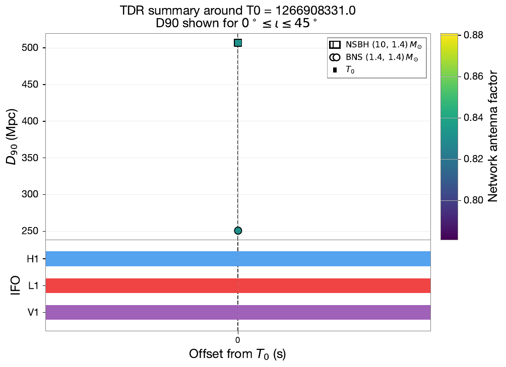
The one-bin scan above runs the repository’s normal trigger pipeline: it determines the observing run, loads public detector strain, estimates PSDs, creates the reference waveform injections, calls pycbc_optimal_snr, computes the BNS TDR map, evaluates BNS/NSBH efficiency curves, and writes JSON/PDF products. The directory is split into scan_t0p0000/ (the trigger-time result) and the shared gwosc_cache/.
# Read the pipeline's decision record: online status alone is not sufficient; strain and PSD must both be usable.
ifo_report = json.loads((RUN_DIR / "ifos_used.json").read_text())
online_ifos = ifo_report["used_ifos"]
status_rows = [
    {
        "IFO": ifo,
        "GWOSC strain available": status["strain_available"],
        "PSD valid": status["psd_ok"],
        "Used by TDR": status["usable"],
        "Reason": status["reason"],
    }
    for ifo, status in ifo_report["ifo_status"].items()
]
display(pd.DataFrame(status_rows).set_index("IFO"))
print("Network used by this run:", online_ifos)
print("TDR status record:", RUN_DIR / "ifos_used.json")
| GWOSC strain available | PSD valid | Used by TDR | Reason | |
|---|---|---|---|---|
| IFO | ||||
| H1 | True | True | True | strain complete and PSD valid |
| L1 | True | True | True | strain complete and PSD valid |
| V1 | True | True | True | strain complete and PSD valid |
Network used by this run: ['H1', 'L1', 'V1']
TDR status record: /Users/samueleronchini/.cache/gw_tdr_tutorial/GRB200228A/scan_t0p0000/ifos_used.json
What “online” means in this run#
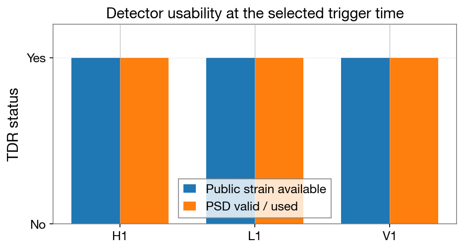
For the trigger-time calculation, TDR reports an IFO as usable when its configured public strain segment is available and its PSD passes validation. This is the pipeline’s data-usability decision; it is not an independent detector-state or full observing-duty-cycle query. The following compact chart visualizes the exact flags in TDR’s own ifos_used.json, and the saved combined PDF is the pipeline’s summary plot.
# Compare strain availability with valid-PSD status for each detector.
ifo_names = list(ifo_report["ifo_status"])
x = np.arange(len(ifo_names))
strain_ok = [ifo_report["ifo_status"][ifo]["strain_available"] for ifo in ifo_names]
psd_ok = [ifo_report["ifo_status"][ifo]["psd_ok"] for ifo in ifo_names]
fig, ax = plt.subplots(figsize=(7, 3.5))
ax.bar(x - 0.18, strain_ok, width=0.36, label="Public strain available")
ax.bar(x + 0.18, psd_ok, width=0.36, label="PSD valid / used")
ax.set(xticks=x, xticklabels=ifo_names, yticks=[0, 1], yticklabels=["No", "Yes"], ylim=(0, 1.2), ylabel="TDR status")
ax.set_title("Detector usability at the selected trigger time")
ax.legend()
ax.grid(axis="y", alpha=0.25)
status_plot = RUN_DIR / "ifo_usability.png"
fig.savefig(status_plot, dpi=150, bbox_inches="tight")
plt.close(fig)
display(Image(filename=str(status_plot)))

# Include TDR's own combined summary plot when the pipeline produced it.
summary_pdf = OUTPUT_ROOT / "D90_and_IFO_windows_combined.pdf"
if summary_pdf.is_file():
    show_pdf(summary_pdf)
2.3 Inspect the detector noise used in the calculation#
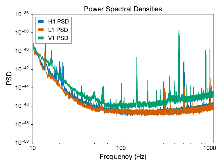
TDR estimates each PSD from the downloaded strain using the production Welch configuration (16 s segments, 8 s overlap), validates and saves a two-column frequency/PSD file, then passes those files to pycbc_optimal_snr. Here we reload those exact PSD files into the repository’s plotting wrapper and call its plot_psd function.
# Load each selected detector's PSD and delegate the production plot to TDR.
psd_objects = [
    PSDWrapper(np.loadtxt(RUN_DIR / f"{ifo.lower()}_psd.txt"))
    for ifo in online_ifos
]
tdr_aux.plot_psd(psd_objects, str(RUN_DIR), ifos=online_ifos)
show_pdf(RUN_DIR / "psd_plot.pdf")
2.4 Plot the live network antenna response#
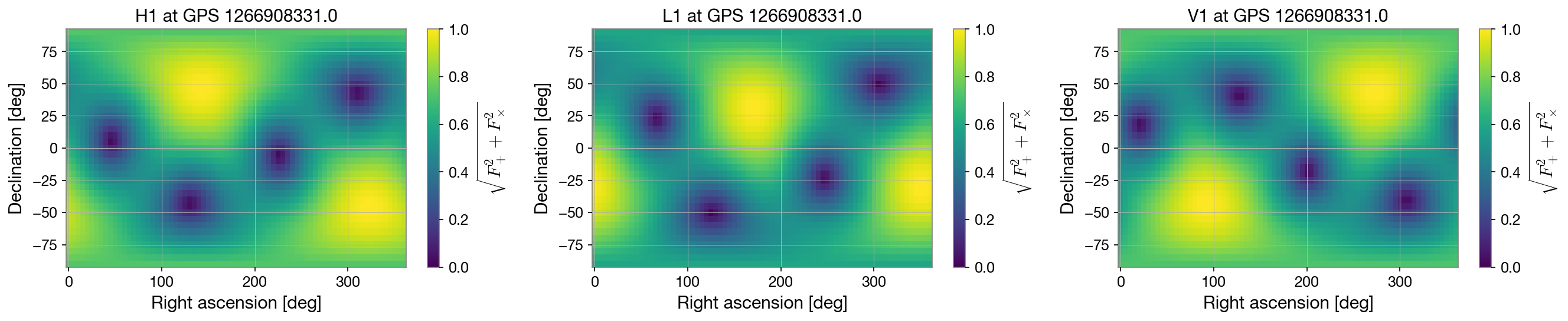
The plots use PyCBC Detector.antenna_pattern, the same detector geometry used by the TDR distance-rescaling calculations, evaluated at the GRB trigger time. Each panel shows \(\sqrt{F_+^2+F_\times^2}\) for polarization angle \(\psi=0\); it is not yet the complete source response, which also weights \(F_+\) and \(F_\times\) by inclination and polarization. compute_antennamap is TDR’s network helper and selects the sky direction maximizing its summed \(F_+^2+F_\times^2\) criterion for the reference injections. The notebook also computes a descriptive network antenna factor at the best sampled direction in the localization; the pipeline itself consumes the sampled sky positions directly.
# Evaluate PyCBC antenna response over a sky grid, at the trigger time, for currently usable IFOs.
ra_axis = np.linspace(0, 2 * np.pi, 73)
dec_axis = np.linspace(-np.pi / 2, np.pi / 2, 37)
ra_mesh, dec_mesh = np.meshgrid(ra_axis, dec_axis)
fig, axes = plt.subplots(1, len(online_ifos), figsize=(6 * len(online_ifos), 3.8), squeeze=False)

for ax, ifo in zip(axes[0], online_ifos):
    detector = Detector(ifo)
    antenna_values = np.vectorize(detector.antenna_pattern, otypes=[float, float])(
        ra_mesh, dec_mesh, 0.0, T0
    )
    f_plus, f_cross = antenna_values
    response = np.hypot(f_plus, f_cross)
    image = ax.pcolormesh(np.rad2deg(ra_mesh), np.rad2deg(dec_mesh), response, shading="auto", vmin=0, vmax=1)
    ax.set(title=f"{ifo} at GPS {T0:.1f}", xlabel="Right ascension [deg]", ylabel="Declination [deg]")
    fig.colorbar(image, ax=ax, label=r"$\sqrt{F_+^2+F_\times^2}$")

# Reuse TDR helpers to sample the GRB localization and summarize its antenna factor.
ra_best, dec_best = tdr_aux.compute_antennamap(online_ifos, T0)
ra_samples, dec_samples, skymap = choose_localization_samples(
    None, None, str(SKYMAP_FILE), ra_best, dec_best
)
def localization_antenna_factor(online_ifos, t0, ra_samples, dec_samples):
    ra_samples = np.asarray(ra_samples, dtype=float).reshape(-1)
    dec_samples = np.asarray(dec_samples, dtype=float).reshape(-1)
    if ra_samples.size == 0 or ra_samples.shape != dec_samples.shape:
        raise ValueError("RA and declination samples must be nonempty arrays of equal length.")
    if not online_ifos:
        raise ValueError("At least one detector is required to calculate a network antenna factor.")

    network_response_sq = np.zeros(ra_samples.shape, dtype=float)
    for ifo in online_ifos:
        f_plus, f_cross = np.vectorize(
            Detector(ifo).antenna_pattern, otypes=[float, float]
        )(ra_samples, dec_samples, 0.0, t0)
        network_response_sq += f_plus**2 + f_cross**2

    best_index = int(np.argmax(network_response_sq))
    return {
        "antenna_factor": float(np.sqrt(network_response_sq[best_index] / len(online_ifos))),
        "antenna_factor_mode": "max_over_grb_skymap_samples",
        "antenna_factor_ra_deg": float(np.rad2deg(ra_samples[best_index]) % 360.0),
        "antenna_factor_dec_deg": float(np.rad2deg(dec_samples[best_index])),
        "antenna_factor_definition": "sqrt(sum_i(Fplus_i^2 + Fcross_i^2) / N_ifo)",
    }

antenna_info = localization_antenna_factor(online_ifos, T0, ra_samples, dec_samples)
print("TDR antenna-max direction [deg]:", np.rad2deg(ra_best), np.rad2deg(dec_best))
print("TDR antenna factor over the sampled GRB localization:", antenna_info)
plt.tight_layout()
antenna_plot = RUN_DIR / "ifo_antenna_response.png"
fig.savefig(antenna_plot, dpi=150, bbox_inches="tight")
plt.close(fig)
display(Image(filename=str(antenna_plot)))
TDR antenna-max direction [deg]: 168.75 38.68218745348943
TDR antenna factor over the sampled GRB localization: {'antenna_factor': 0.8319250844324213, 'antenna_factor_mode': 'max_over_grb_skymap_samples', 'antenna_factor_ra_deg': 347.6953125, 'antenna_factor_dec_deg': -39.45089470914607, 'antenna_factor_definition': 'sqrt(sum_i(Fplus_i^2 + Fcross_i^2) / N_ifo)'}
2.5 Recompute efficiency curves for the selected inclination prior#
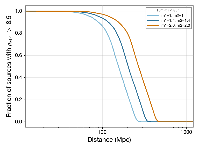
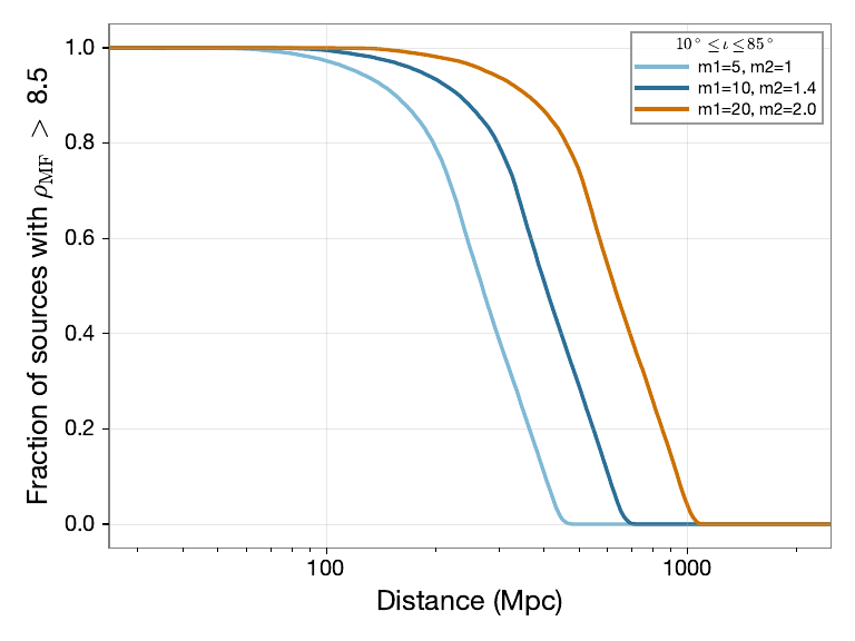
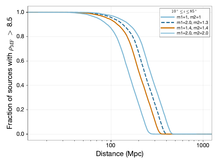
The CLI and the following compute_range call use exactly one interval: \(IOTA\_MIN\_DEG\)–\(IOTA\_MAX\_DEG\) (default \(0\)–\(45^\circ\)). Edit these two settings in §2.2 to choose a different range; TDR will not evaluate additional 30°, 45°, or 90° cases. We recompute the selected run’s efficiency curves from the saved optimal-SNR HDF files produced by the actual PyCBC injections, then show its tables and curves below.
For each reference injection, compute_range rescales detector SNR using PyCBC effective distances at the source and reference locations, combines detector contributions in quadrature, samples the selected inclination prior, and measures the fraction above threshold as distance increases. \(D_{90}\) is the distance where that fraction reaches 90%. The repository’s mf statistic is its matched-filter-like conversion from optimal SNR; it is not a measured search FAR.
# Translate the selected degree interval to radians and choose the requested SNR convention.
IOTA_MIN_DEG = 10.0  # Set the single inclination prior used in this run.
IOTA_MAX_DEG = 85.0
if not 0 <= IOTA_MIN_DEG < IOTA_MAX_DEG <= 90:
    raise ValueError("Choose one valid inclination interval: 0 <= IOTA_MIN_DEG < IOTA_MAX_DEG <= 90 degrees.")

iota_ranges = [{
    "label": f"{IOTA_MIN_DEG:g}-{IOTA_MAX_DEG:g}",
    "iota_min": np.deg2rad(IOTA_MIN_DEG),
    "iota_max": np.deg2rad(IOTA_MAX_DEG),
}]
selected_snrs = "matched_filter" if SNR_STATISTIC == "mf" else "optimal"
np.random.seed(12345 + int(round(T0)))
# Calculate the BNS sky map and all configured BNS/NSBH efficiency curves with production routines.
range_map = Path(tdr_aux.compute_map(
    "bns", "1.4", "1.4", online_ifos, str(RUN_DIR),
    iota_ranges[0]["iota_min"], iota_ranges[0]["iota_max"],
    SNR_THRESHOLD, selected_snrs,
))
tdr_aux.compute_range(
    ra_samples,
    dec_samples,
    online_ifos,
    CHIRP_MASSES,
    str(RUN_DIR),
    iota_ranges,
    SNR_THRESHOLD,
    selected_snrs,
)
print(f"Computed one inclination prior: {IOTA_MIN_DEG:g}-{IOTA_MAX_DEG:g} deg")
print("Selected-prior TDR map, efficiency curves, and refreshed result JSON written under", RUN_DIR)
setting the output map dtype to [dtype('float64')]
Computed one inclination prior: 10-85 deg
Selected-prior TDR map, efficiency curves, and refreshed result JSON written under /Users/samueleronchini/.cache/gw_tdr_tutorial/GRB200228A/scan_t0p0000
# Flatten the nested production JSON into a display-ready row per system and inclination prior.
def read_tdr_table(path):
    """Flatten the production JSON schema into one row per mass/prior pair."""
    payload = json.loads(Path(path).read_text())
    rows = []
    for source_class, systems in payload.items():
        for mass_label, entry in systems.items():
            for prior_label, value in entry["tdr"].items():
                rows.append({
                    "Source class": source_class.upper(),
                    "Mass pair": mass_label,
                    "Inclination prior": prior_label,
                    "IFO network": ",".join(entry.get("online_ifos", [])),
                    "SNR statistic": entry.get("snr_statistic", SNR_STATISTIC),
                    "Threshold": entry.get("snr_threshold", SNR_THRESHOLD),
                    "D90 [Mpc]": value["D90_Mpc"],
                })
    return pd.DataFrame(rows)

bns_table = read_tdr_table(RUN_DIR / "results_bns.json")
nsbh_table = read_tdr_table(RUN_DIR / "results_nsbh.json")
tdr_table = pd.concat([bns_table, nsbh_table], ignore_index=True)
display(tdr_table)
| Source class | Mass pair | Inclination prior | IFO network | SNR statistic | Threshold | D90 [Mpc] | |
|---|---|---|---|---|---|---|---|
| 0 | BNS | m1=1, m2=1 | 10-85 | H1,L1,V1 | matched_filter | 8.5 | 89.682336 |
| 1 | BNS | m1=1.4, m2=1.4 | 10-85 | H1,L1,V1 | matched_filter | 8.5 | 117.186559 |
| 2 | BNS | m1=2.0, m2=2.0 | 10-85 | H1,L1,V1 | matched_filter | 8.5 | 154.699299 |
| 3 | NSBH | m1=5, m2=1 | 10-85 | H1,L1,V1 | matched_filter | 8.5 | 155.229373 |
| 4 | NSBH | m1=10, m2=1.4 | 10-85 | H1,L1,V1 | matched_filter | 8.5 | 233.246425 |
| 5 | NSBH | m1=20, m2=2.0 | 10-85 | H1,L1,V1 | matched_filter | 8.5 | 361.394866 |
These tables are flattened from the current run’s results_bns.json and results_nsbh.json; they contain only the single inclination interval selected by IOTA_MIN_DEG and IOTA_MAX_DEG. NSBH values follow the repository’s EOS-averaging convention. The efficiency curves below are generated by the repository’s compute_range for that same run and prior. Do not read the result as an astrophysical exclusion without a corresponding search analysis.
# Display the efficiency curves generated by TDR for the selected mass classes.
for filename in ("bns_targeted_range.pdf", "nsbh_targeted_range.pdf"):
    print(filename)
    show_pdf(RUN_DIR / filename)
bns_targeted_range.pdf
nsbh_targeted_range.pdf
2.6 Inspect the TDR sky map#
Here compute_map("bns", 1.4, 1.4, ...) evaluates the 90%-detectable distance over TDR’s HEALPix grid using the actual reference-SNR HDF file, detector geometry, trigger time, the same single user-selected inclination interval as the table/curves, and the SNR threshold. plot_final renders that FITS map in the same format used by the repository. The map is a sensitivity map over sky position, not a posterior probability map.
# Load and plot the production HEALPix TDR map with its localization context.
range_map = RUN_DIR / "range_map_bns_m1_1.4_m2_1.4.fits"
assert range_map.is_file(), f"TDR map not found: {range_map}"
tdr_aux.plot_final(
    str(RUN_DIR), str(range_map), str(skymap),
    [ra_samples, dec_samples],
    iota_ranges[0]["iota_min"], iota_ranges[0]["iota_max"],
)
show_pdf(RUN_DIR / "range_map_bns_m1_1.4_m2_1.4.pdf")
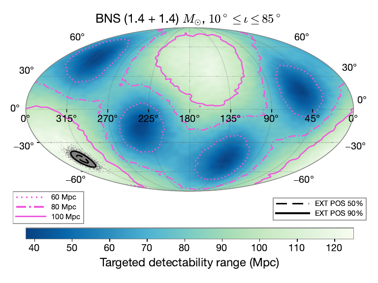
2.7 Exercise: compare another source sky map#
The main calculation already propagates the paper’s GRB 200228A localization through TDR. To compare another real GRB/source localization, supply its HEALPix FITS file (with PROB or PROBABILITY). The production helper choose_localization_samples delegates to TDR’s map_samples, which normalizes pixel probabilities and draws sky samples. The code below passes those RA/Dec draws to production compute_range, saves results separately, and uses TDR’s plot_final to overlay the alternate localization on the TDR map.
Exercise: compare the paper’s GRB map-conditioned table with a second sky-map-conditioned table. How does probability on less-sensitive parts of the sky change the fraction-versus-distance curves? Preserve the paired result directories to compare both outputs.
# Set an alternate real HEALPix FITS map here to repeat the source-localization calculation.
ALTERNATE_SKYMAP_FILE = None  # Set to Path("/path/to/another_localization.fits") to run this exercise.

if ALTERNATE_SKYMAP_FILE is None:
    print("Exercise not run: set ALTERNATE_SKYMAP_FILE to another real HEALPix FITS localization.")
else:
    skymap_path = Path(ALTERNATE_SKYMAP_FILE).expanduser()
    if not skymap_path.is_file():
        raise FileNotFoundError(skymap_path)
    # Preserve the cached waveform/SNR references; recompute only localization-dependent quantities.
    ra_samples, dec_samples, skymap = choose_localization_samples(
        None, None, str(skymap_path), ra_best, dec_best
    )
    skymap_dir = OUTPUT_ROOT / f"skymap_{skymap_path.stem}"
    skymap_dir.mkdir(parents=True, exist_ok=True)
    shutil.copytree(RUN_DIR / "results", skymap_dir / "results", dirs_exist_ok=True)
    antenna_info_skymap = localization_antenna_factor(
        online_ifos, T0, ra_samples, dec_samples
    )
    print("Alternate-map antenna factor:", antenna_info_skymap)
    np.random.seed(12345 + int(round(T0)))
    tdr_aux.compute_range(
        ra_samples, dec_samples, online_ifos, CHIRP_MASSES, str(skymap_dir),
        iota_ranges, SNR_THRESHOLD,
        "matched_filter" if SNR_STATISTIC == "mf" else "optimal",
    )
    tdr_aux.plot_final(
        str(skymap_dir), str(range_map), str(skymap), [ra_samples, dec_samples],
        iota_ranges[0]["iota_min"], iota_ranges[0]["iota_max"],
    )
    display(read_tdr_table(skymap_dir / "results_bns.json"))
    show_pdf(skymap_dir / "range_map_bns_m1_1.4_m2_1.4.pdf")
Exercise not run: set ALTERNATE_SKYMAP_FILE to another real HEALPix FITS localization.
2.8 Exercise: propagate joint mass, inclination, and sky samples#
The current production calculation samples isotropic inclination within a requested interval, reads a fixed set of reference mass-pair injections, and accepts sky samples independently from a localization map. It does not accept arbitrary correlated posterior rows. A research extension should preserve each posterior tuple \((m_1,m_2,\iota,\mathrm{RA},\mathrm{Dec})\) and its weight rather than drawing each marginal independently.
Start with a CSV of posterior samples with columns m1, m2, iota_rad, ra_deg, dec_deg and optional weight. The next cell creates an illustrative sample set by drawing an independent Gaussian for every required parameter; these are not measured GRB posterior samples and have no cross-parameter correlations. Change the means and widths, or replace the generated CSV with real paired posterior samples. The following cells validate and resample whole rows, plot their parameter marginals and joint mass/sky distributions, then calculate a custom efficiency curve and TDR map. The custom calculation uses the nearest available reference mass pair and an inclination grid reweighted by the supplied angle distribution; it is an approximation, not a full arbitrary-mass injection run. The grid marginal treats inclination independently of mass and sky position, so correlations with those parameters are not retained. A useful extension is to make the production waveform/SNR references support arbitrary sampled masses and preserve all joint posterior correlations.
Do not pass these samples to the current compute_range as if it already accepted them: its signature and sampler do not.
# Illustrative independent Gaussian marginals; these are not measured GRB posterior samples.
# Edit the means/centers and sigmas below to choose each distribution. Masses use solar masses;
# inclination, RA, and Dec settings use degrees. Set either sky center to None to use the GRB
# localization center. RA_SIGMA_DEG is the east-west angular spread; DEC_SIGMA_DEG is the Dec spread.
M1_MEAN, M1_SIGMA = 10.46, 0.12
M2_MEAN, M2_SIGMA = 1.30, 0.10
IOTA_MEAN_DEG, IOTA_SIGMA_DEG = 30.0, 10.0
RA_CENTER_DEG, DEC_CENTER_DEG = 45, 45
RA_SIGMA_DEG, DEC_SIGMA_DEG = 2.0, 2.0
N_GAUSSIAN_SAMPLES = 5_000
rng = np.random.default_rng(20261008)

# Rejection-sample a Gaussian so every generated value obeys the physical/configured bounds.
def truncated_normal(mean, sigma, size, lower, upper, rng):
    draws = np.empty(size)
    filled = 0
    while filled < size:
        candidates = rng.normal(mean, sigma, size=max(100, 2 * (size - filled)))
        accepted = candidates[(candidates >= lower) & (candidates <= upper)]
        count = min(len(accepted), size - filled)
        draws[filled:filled + count] = accepted[:count]
        filled += count
    return draws

# Draw component masses jointly and retain only physical mass ordering.
m1_draws = []
m2_draws = []
while len(m1_draws) < N_GAUSSIAN_SAMPLES:
    batch_size = 2 * (N_GAUSSIAN_SAMPLES - len(m1_draws))
    #larger mass is m1, smaller mass is m2; both are truncated to physical ranges.
    m1_batch = rng.normal(M1_MEAN, M1_SIGMA, batch_size)
    m2_batch = rng.normal(M2_MEAN, M2_SIGMA, batch_size)
    valid = (
        (m1_batch >= 1.0) & (m1_batch <= 25.0)
        & (m2_batch >= 1.0) & (m2_batch <= 2.0)
        & (m1_batch >= m2_batch)
    )
    m1_draws.extend(m1_batch[valid].tolist())
    m2_draws.extend(m2_batch[valid].tolist())
m1_draws = np.asarray(m1_draws[:N_GAUSSIAN_SAMPLES])
m2_draws = np.asarray(m2_draws[:N_GAUSSIAN_SAMPLES])

# Draw component masses, sky position, and inclination within their chosen supports.
# Center the sky prior on the circular mean of the GRB localization samples.
ra_center = (
    np.arctan2(np.mean(np.sin(ra_samples)), np.mean(np.cos(ra_samples))) % (2 * np.pi)
    if RA_CENTER_DEG is None else np.deg2rad(RA_CENTER_DEG) % (2 * np.pi)
)
dec_center = float(np.mean(dec_samples)) if DEC_CENTER_DEG is None else np.deg2rad(DEC_CENTER_DEG)
ra_sigma = np.deg2rad(RA_SIGMA_DEG) / max(abs(np.cos(dec_center)), 0.1)  # convert east-west spread to RA-coordinate spread
ra_draws = (ra_center + rng.normal(0.0, ra_sigma, N_GAUSSIAN_SAMPLES)) % (2 * np.pi)
dec_draws = truncated_normal(dec_center, np.deg2rad(DEC_SIGMA_DEG), N_GAUSSIAN_SAMPLES, -np.pi / 2, np.pi / 2, rng)
iota_draws = truncated_normal(np.deg2rad(IOTA_MEAN_DEG), np.deg2rad(IOTA_SIGMA_DEG), N_GAUSSIAN_SAMPLES, 0.0, np.pi / 2, rng)

# Save the source tuples and inspect their one-dimensional distributions.
gaussian_samples = pd.DataFrame({
    "m1": m1_draws,
    "m2": m2_draws,
    "iota_rad": iota_draws,
    "ra_deg": np.rad2deg(ra_draws),
    "dec_deg": np.rad2deg(dec_draws),
})
GAUSSIAN_SAMPLE_FILE = OUTPUT_ROOT / "gaussian_joint_source_samples.csv"
gaussian_samples.to_csv(GAUSSIAN_SAMPLE_FILE, index=False)

fig, axes = plt.subplots(1, 5, figsize=(16, 3))
labels = (r"$m_1$ [$M_\odot$]", r"$m_2$ [$M_\odot$]", r"$\iota$ [rad]", "RA [deg]", "Dec [deg]")
for ax, column, label in zip(axes, gaussian_samples.columns, labels):
    ax.hist(gaussian_samples[column], bins=30, density=True, color="steelblue", alpha=0.8)
    ax.set_xlabel(label)
    ax.set_ylabel("Density")
fig.tight_layout()
display(fig)
plt.close(fig)
print(f"Created {len(gaussian_samples)} Gaussian source samples: {GAUSSIAN_SAMPLE_FILE}")
display(gaussian_samples.head())
<Figure size 1600x300 with 5 Axes>
Created 5000 Gaussian source samples: /Users/samueleronchini/.cache/gw_tdr_tutorial/GRB200228A/gaussian_joint_source_samples.csv
| m1 | m2 | iota_rad | ra_deg | dec_deg | |
|---|---|---|---|---|---|
| 0 | 10.458762 | 1.232542 | 0.467885 | 47.082266 | 45.494213 |
| 1 | 10.298313 | 1.344980 | 0.357804 | 47.820291 | 47.354326 |
| 2 | 10.732957 | 1.394992 | 0.511255 | 44.609148 | 45.737857 |
| 3 | 10.443762 | 1.197908 | 0.397474 | 43.146574 | 44.332533 |
| 4 | 10.456127 | 1.187059 | 0.383372 | 44.998203 | 47.164176 |
# Select the source-posterior file; optionally provide a separate inclination-only prior file.
POSTERIOR_CSV = GAUSSIAN_SAMPLE_FILE  # Replace with a real posterior CSV to use external samples.
INCLINATION_PRIOR_CSV = None  # Optional CSV with iota_deg or iota_rad and optional weight columns.
joint_draws = None

if POSTERIOR_CSV is None:
    print("Exercise not run: provide real, paired source-posterior samples in a CSV.")
else:
    posterior = pd.read_csv(Path(POSTERIOR_CSV).expanduser())
    # Validate required fields, inclination bounds, and optional sample weights before resampling.
    required = {"m1", "m2", "iota_rad", "ra_deg", "dec_deg"}
    missing = required - set(posterior.columns)
    if missing:
        raise ValueError(f"Posterior is missing required columns: {sorted(missing)}")
    inclination_samples = posterior["iota_rad"].to_numpy(dtype=float)
    if not np.all(np.isfinite(inclination_samples)) or np.any((inclination_samples < 0) | (inclination_samples > np.pi / 2)):
        raise ValueError("Posterior iota_rad values must be finite and between 0 and pi/2 radians.")
    weights = posterior["weight"].to_numpy(dtype=float) if "weight" in posterior else np.ones(len(posterior))
    if len(posterior) == 0 or not np.all(np.isfinite(weights)) or np.any(weights < 0) or weights.sum() <= 0:
        raise ValueError("Posterior must have rows and finite, nonnegative weights with positive sum.")
    # Resample complete rows so correlations in a supplied joint posterior remain paired.
    rng = np.random.default_rng(417)
    row_indices = rng.choice(len(posterior), size=10_000, replace=True, p=weights / weights.sum())
    joint_draws = posterior.iloc[row_indices].reset_index(drop=True)
    print(f"Resampled {len(joint_draws)} complete joint tuples; correlations are retained.")
    display(joint_draws.head())
    print("Next: extend the production injection/reference-SNR and weighted efficiency calculation as specified above.")
Resampled 10000 complete joint tuples; correlations are retained.
| m1 | m2 | iota_rad | ra_deg | dec_deg | |
|---|---|---|---|---|---|
| 0 | 10.450149 | 1.343145 | 0.480540 | 41.892475 | 50.645293 |
| 1 | 10.496158 | 1.291303 | 0.671820 | 46.051865 | 42.869765 |
| 2 | 10.466605 | 1.321608 | 0.509514 | 43.847301 | 42.882824 |
| 3 | 10.372715 | 1.361028 | 0.359613 | 42.096729 | 43.895231 |
| 4 | 10.424084 | 1.388577 | 0.453238 | 45.215469 | 46.728877 |
Next: extend the production injection/reference-SNR and weighted efficiency calculation as specified above.
Plot the custom source samples#
These plots show the selected joint sample set (the Gaussian example by default, or the CSV you configured above). The marginals summarize each parameter; the scatter panels show paired values from the same rows. They visualize the source samples only, not a TDR efficiency curve or sky sensitivity map.
# Visualize the resampled parameter marginals and paired mass/sky samples before using them downstream.
if joint_draws is None:
    print("No custom samples to plot. Set POSTERIOR_CSV to a valid sample CSV.")
else:
    fig, axes = plt.subplots(2, 3, figsize=(14, 8))
    for ax, column, label in zip(
        axes[0],
        ("m1", "m2", "iota_rad"),
        (r"$m_1$ [$M_\odot$]", r"$m_2$ [$M_\odot$]", r"$\iota$ [rad]"),
    ):
        ax.hist(joint_draws[column], bins=35, density=True, color="steelblue", alpha=0.8)
        ax.set_xlabel(label)
        ax.set_ylabel("Density")
        ax.grid(alpha=0.2)

    mass_scatter = axes[1, 0].scatter(
        joint_draws["m1"], joint_draws["m2"], c=joint_draws["iota_rad"],
        s=8, alpha=0.35, cmap="viridis",
    )
    axes[1, 0].set(xlabel=r"$m_1$ [$M_\odot$]", ylabel=r"$m_2$ [$M_\odot$]", title="Paired component masses")
    fig.colorbar(mass_scatter, ax=axes[1, 0], label=r"$\iota$ [rad]")

    sky_scatter = axes[1, 1].scatter(
        joint_draws["ra_deg"], joint_draws["dec_deg"], c=joint_draws["iota_rad"],
        s=8, alpha=0.35, cmap="viridis",
    )
    axes[1, 1].set(xlabel="RA [deg]", ylabel="Dec [deg]", title="Paired sky samples")
    # Zoom to a 3-sigma window around the configured Gaussian sky center.
    ra_center_deg = np.rad2deg(ra_center)
    dec_center_deg = np.rad2deg(dec_center)
    ra_half_width_deg = 3 * np.rad2deg(ra_sigma)
    dec_half_width_deg = 3 * DEC_SIGMA_DEG
    axes[1, 1].set_xlim(ra_center_deg - ra_half_width_deg, ra_center_deg + ra_half_width_deg)
    axes[1, 1].set_ylim(dec_center_deg - dec_half_width_deg, dec_center_deg + dec_half_width_deg)
    fig.colorbar(sky_scatter, ax=axes[1, 1], label=r"$\iota$ [rad]")
    axes[1, 2].axis("off")
    fig.tight_layout()
    joint_plot_path = OUTPUT_ROOT / "joint_source_sample_distributions.png"
    fig.savefig(joint_plot_path, dpi=150, bbox_inches="tight")
    plt.close(fig)
    display(Image(filename=str(joint_plot_path)))
    print(f"Sample plots saved to {joint_plot_path}")
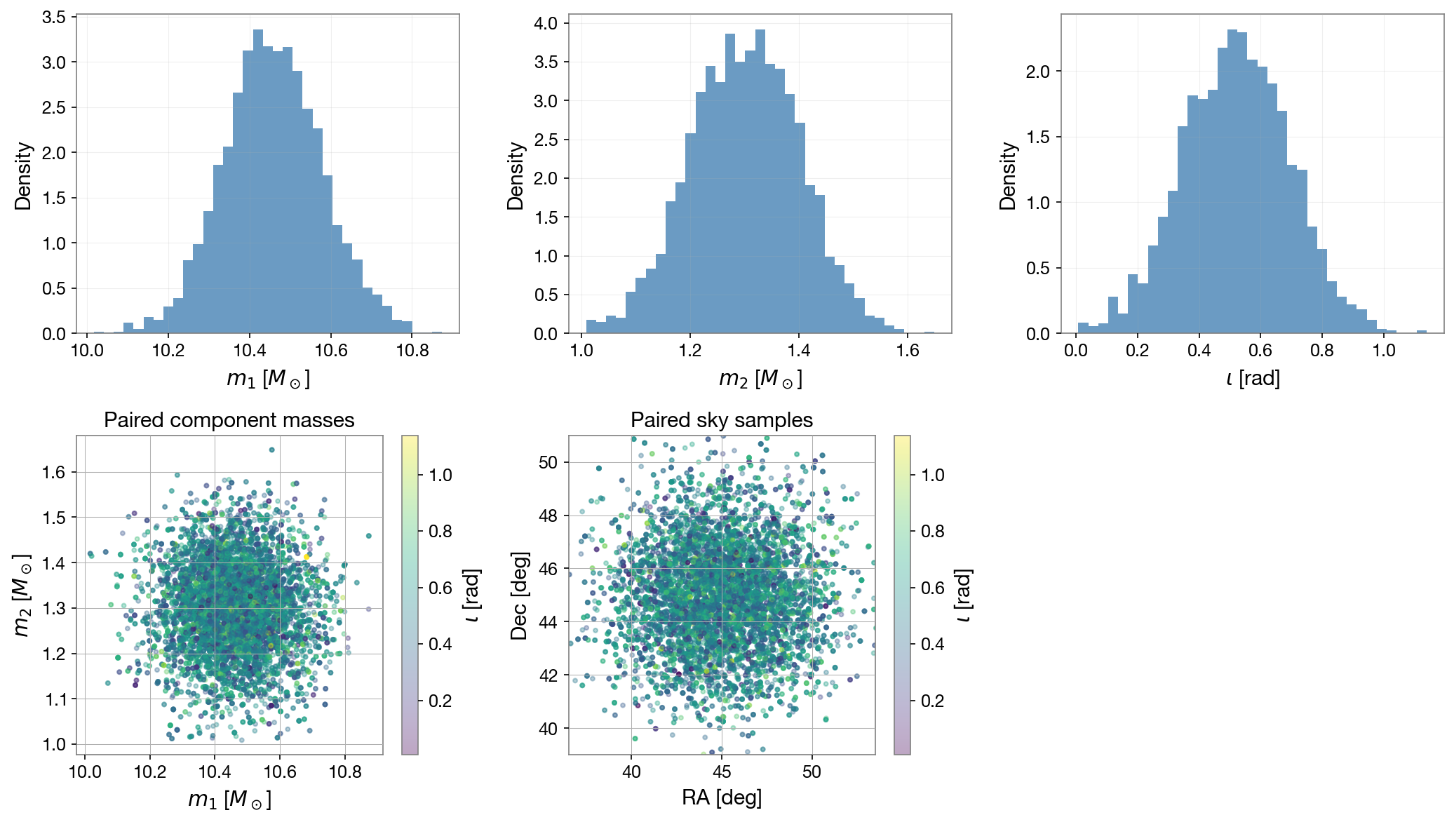
Sample plots saved to /Users/samueleronchini/.cache/gw_tdr_tutorial/GRB200228A/joint_source_sample_distributions.png
Inclination-grid marginalization of efficiency and TDR map#
This calculation evaluates the response on a uniform inclination grid from 0° through 90° (5° spacing), regardless of the interval selected for the main production run. It then assigns each grid point the probability mass of the user-supplied inclination distribution in that grid cell. By default, the angle distribution comes from iota_rad in POSTERIOR_CSV; optionally, set INCLINATION_PRIOR_CSV to a CSV containing iota_deg or iota_rad and an optional weight column. All supplied angles must be finite and in [0°, 90°]. The weighted grid is used consistently for the efficiency curve and marginalized TDR sky map.
The inclination marginal is applied independently of sampled masses and sky position; correlations between inclination, mass, and sky position are therefore not preserved. The TDR checkout does not yet accept arbitrary joint posterior rows directly. Its saved BNS reference injections are available only at \((1,1)\), \((1.4,1.4)\), and \((2,2)\,M_\odot\); this notebook uses the nearest reference mass pair for each sampled mass. This is a discrete-template approximation, not a fresh waveform or SNR evaluation at every continuous sampled mass.
Operational sequence#
Assign a mass reference. For each input row \((m_1,m_2,\mathrm{RA},\mathrm{Dec})\), select the nearest of the three cached BNS reference mass pairs. The corresponding per-IFO optimal SNR and reference effective distance are read from the pipeline results. Thus, changing the input masses changes which cached waveform reference is used, but does not generate new waveforms.
Build the inclination prior on a grid. The response is evaluated at 19 fixed angles, \(0^\circ,5^\circ,\ldots,90^\circ\). The input inclination samples (and their optional
weightvalues) are binned into cells centered on these grid angles.Calculate source-sample horizons. For every resampled source row, evaluate PyCBC
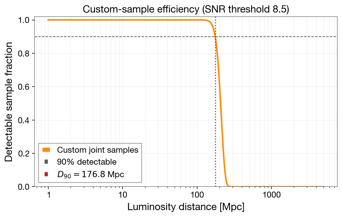
Detector.effective_distanceat its own sky coordinates and polarization, at each inclination-grid angle. Scale each cached detector SNR by \(D_{\mathrm{eff,ref}}/D_{\mathrm{eff}}\) and combine detector SNRs in quadrature. If requested, convert the network optimal SNR to the matched-filter statistic. For threshold \(\rho_*\), each combination has horizon \(D_{\mathrm{hor}}=100\,\mathrm{Mpc}\,\rho/\rho_*\). The code draws polarization uniformly and holds it fixed across the inclination grid for a given row.Form the efficiency curve and \(D_{90}\). At every trial distance \(D\), count a row/grid-angle combination as detectable when \(D_{\mathrm{hor}}>D\). Average these indicators over the source rows and inclination-grid weights: \(\epsilon(D)=N^{-1}\sum_{j=1}^{N}\sum_k w_k\,\mathbf{1}(D_{\mathrm{hor},jk}>D)\). The plotted efficiency decreases with distance; \(D_{90}\) is the first point on the distance grid where \(\epsilon(D)<0.9\).
Build the sky map. For each HEALPix pixel, select up to 500 source rows (without replacement) and recalculate their detector response at that pixel, across the same inclination grid and prior weights. The pixel value is the weighted 10th percentile of those horizons: at that distance, 90% of the weighted combinations reach the SNR threshold.
The joint-sample input is first resampled according to its optional row weight, but the inclination prior is then marginalized separately and independently for every row. Consequently, the current calculation preserves the sampled mass/sky tuples but does not preserve correlations of inclination with mass or sky. The map’s up-to-500 rows are selected uniformly from this already-resampled set.
# Evaluate the custom-sample efficiency and map by reweighting a uniform 0-90 degree inclination grid.
if joint_draws is None:
    print("No joint samples available. Set POSTERIOR_CSV and rerun the sample cells first.")
else:
    from targ_ac_git.aux_snr_mf import _convert_opt_to_mf_snr, _read_optimal_snr_file

    # Choose the nearest cached BNS mass reference for each sampled mass pair (a discrete approximation).
    reference_templates = [(1.0, 1.0, "1", "1"), (1.4, 1.4, "1.4", "1.4"), (2.0, 2.0, "2.0", "2.0")]
    reference_masses = np.array([[item[0], item[1]] for item in reference_templates])
    reference_data = []
    sample_masses = joint_draws[["m1", "m2"]].to_numpy(dtype=float)
    template_index = np.argmin(
        np.sum(((sample_masses[:, None, :] - reference_masses[None, :, :]) / 0.4) ** 2, axis=2),
        axis=1,
    )

    custom_detectors = {ifo: Detector(ifo) for ifo in online_ifos}
    for m1_ref, m2_ref, m1_tag, m2_tag in reference_templates:
        reference_file = RUN_DIR / "results" / f"results_bns_m1_{m1_tag}_m2_{m2_tag}.hdf"
        ref_ifos, ref_snr, ref_ra, ref_dec, ref_t0 = _read_optimal_snr_file(str(reference_file))
        if sorted(ref_ifos) != sorted(online_ifos):
            raise ValueError(f"Detector mismatch in reference file {reference_file}: {ref_ifos}")
        reference_data.append({
            "snr": {ifo: float(np.asarray(ref_snr[ifo]).reshape(-1)[0]) for ifo in ref_ifos},
            "ref_eff": {
                ifo: float(custom_detectors[ifo].effective_distance(100.0, ref_ra, ref_dec, 0.0, ref_t0, 0.0))
                for ifo in ref_ifos
            },
        })

    # Scale each reference optimal SNR by the PyCBC effective-distance ratio and combine IFOs in quadrature.
    def custom_network_snr(ra, dec, iota, polarization, template_ids):
        network_snr_sq = np.zeros(len(template_ids), dtype=float)
        for ifo in online_ifos:
            detector = custom_detectors[ifo]
            effective_distance = np.asarray(
                detector.effective_distance(100.0, ra, dec, polarization, T0, iota),
                dtype=float,
            )
            reference_snr = np.array([reference_data[index]["snr"][ifo] for index in template_ids])
            reference_distance = np.array([reference_data[index]["ref_eff"][ifo] for index in template_ids])
            scale = np.divide(
                reference_distance, effective_distance,
                out=np.zeros_like(effective_distance),
                where=np.isfinite(effective_distance) & (effective_distance > 0),
            )
            network_snr_sq += (reference_snr * scale) ** 2
        return np.sqrt(network_snr_sq)

    custom_rng = np.random.default_rng(20261009)
    sample_ra = np.deg2rad(joint_draws["ra_deg"].to_numpy(dtype=float))
    sample_dec = np.deg2rad(joint_draws["dec_deg"].to_numpy(dtype=float))
    # Bin the user-provided inclination prior onto the uniform grid, then normalize its probability masses.
    inclination_grid_deg = np.linspace(0.0, 90.0, 19)
    iota_grid_size = len(inclination_grid_deg)
    iota_grid = np.deg2rad(inclination_grid_deg)
    angle_edges_deg = np.concatenate(([0.0], (inclination_grid_deg[:-1] + inclination_grid_deg[1:]) / 2, [90.0]))
    if INCLINATION_PRIOR_CSV is None:
        prior_angles_deg = np.rad2deg(joint_draws["iota_rad"].to_numpy(dtype=float))
        prior_source_weights = np.ones(len(prior_angles_deg), dtype=float)
        inclination_prior_label = "POSTERIOR_CSV iota_rad"
    else:
        inclination_prior = pd.read_csv(Path(INCLINATION_PRIOR_CSV).expanduser())
        if "iota_deg" in inclination_prior:
            prior_angles_deg = inclination_prior["iota_deg"].to_numpy(dtype=float)
        elif "iota_rad" in inclination_prior:
            prior_angles_deg = np.rad2deg(inclination_prior["iota_rad"].to_numpy(dtype=float))
        else:
            raise ValueError("INCLINATION_PRIOR_CSV must contain iota_deg or iota_rad.")
        prior_source_weights = inclination_prior["weight"].to_numpy(dtype=float) if "weight" in inclination_prior else np.ones(len(inclination_prior))
        inclination_prior_label = str(INCLINATION_PRIOR_CSV)
    if (len(prior_angles_deg) == 0 or not np.all(np.isfinite(prior_angles_deg))
            or np.any((prior_angles_deg < 0.0) | (prior_angles_deg > 90.0))):
        raise ValueError("Inclination prior angles must be nonempty, finite, and between 0 and 90 degrees.")
    if (not np.all(np.isfinite(prior_source_weights)) or np.any(prior_source_weights < 0.0)
            or prior_source_weights.sum() <= 0.0):
        raise ValueError("Inclination-prior weights must be finite, nonnegative, and have positive sum.")
    inclination_bin_mass, _ = np.histogram(
        prior_angles_deg, bins=angle_edges_deg, weights=prior_source_weights,
    )
    iota_weights = inclination_bin_mass.astype(float) / inclination_bin_mass.sum()
    source_row_count = len(joint_draws)
    sample_polarization = custom_rng.uniform(0.0, 2.0 * np.pi, source_row_count)
    sample_template_ids = template_index
    sample_ra_grid = np.repeat(sample_ra, iota_grid_size)
    sample_dec_grid = np.repeat(sample_dec, iota_grid_size)
    sample_iota_grid = np.tile(iota_grid, source_row_count)
    sample_polarization_grid = np.repeat(sample_polarization, iota_grid_size)
    sample_template_grid = np.repeat(sample_template_ids, iota_grid_size)
    marginal_weights = np.tile(iota_weights / source_row_count, source_row_count)
    marginal_weights /= marginal_weights.sum()
    # Evaluate SNR at each source-sample/grid-angle combination and form its threshold horizon.
    sample_snr_opt = custom_network_snr(
        sample_ra_grid, sample_dec_grid, sample_iota_grid,
        sample_polarization_grid, sample_template_grid,
    )
    if SNR_STATISTIC == "mf":
        sample_snr = _convert_opt_to_mf_snr(sample_snr_opt, len(online_ifos))
    else:
        sample_snr = sample_snr_opt

    sample_horizons = 100.0 * sample_snr / SNR_THRESHOLD
    distance_grid = np.logspace(0, np.log10(5000.0), 1000)
    # At each distance, sum prior weights for samples whose horizon exceeds that distance; D90 is the 90% crossing.
    sample_efficiency = np.sum(
        marginal_weights[:, None] * (sample_horizons[:, None] > distance_grid[None, :]),
        axis=0,
    )
    d90_index = np.flatnonzero(sample_efficiency < 0.9)
    sample_d90 = float(distance_grid[d90_index[0]]) if len(d90_index) else float(distance_grid[-1])

    # Save and display the weighted efficiency curve and the prior weights used in the marginalization.
    fig, ax = plt.subplots(figsize=(7, 4.5))
    ax.plot(distance_grid, sample_efficiency, color="darkorange", lw=2.2, label="Custom joint samples")
    ax.axhline(0.9, color="0.35", ls="--", lw=1, label="90% detectable")
    ax.axvline(sample_d90, color="firebrick", ls=":", lw=1.5, label=rf"$D_{{90}}={sample_d90:.1f}$ Mpc")
    ax.set(xscale="log", xlabel="Luminosity distance [Mpc]", ylabel="Detectable sample fraction", ylim=(0, 1.02))
    ax.set_title(f"Custom-sample efficiency (SNR threshold {SNR_THRESHOLD:g})")
    ax.grid(True, which="both", alpha=0.25)
    ax.legend()
    fig.tight_layout()
    custom_output_dir = OUTPUT_ROOT / "custom_joint_tdr"
    custom_output_dir.mkdir(parents=True, exist_ok=True)
    efficiency_plot_path = custom_output_dir / "custom_sample_efficiency.png"
    fig.savefig(efficiency_plot_path, dpi=160, bbox_inches="tight")
    plt.close(fig)
    display(Image(filename=str(efficiency_plot_path)))
    custom_tdr_table = pd.DataFrame([{
        "Inclination grid [deg]": f"0-90, uniform {inclination_grid_deg[1] - inclination_grid_deg[0]:g} deg spacing",
        "Inclination prior source": inclination_prior_label,
        "Inclination-prior grid weights": np.array2string(iota_weights, precision=3),
        "Inclination grid points": iota_grid_size,
        "Source rows": source_row_count,
        "SNR statistic": SNR_STATISTIC,
        "SNR threshold": SNR_THRESHOLD,
        "Marginalized D90 [Mpc]": sample_d90,
    }])
    display(custom_tdr_table)
    display(pd.DataFrame({"Inclination [deg]": inclination_grid_deg, "Prior probability mass": iota_weights}))
    print(f"Marginalized efficiency curve: {efficiency_plot_path}")

    # At each HEALPix pixel, take the 10th percentile weighted horizon (equivalent to 90% detectability).
    map_rng = np.random.default_rng(20261010)
    map_sample_count = min(500, len(joint_draws))
    map_indices = map_rng.choice(len(joint_draws), size=map_sample_count, replace=False)
    map_polarization = sample_polarization[map_indices]
    map_template_ids = np.repeat(sample_template_ids[map_indices], iota_grid_size)
    map_iota = np.tile(iota_grid, map_sample_count)
    map_polarization = np.repeat(map_polarization, iota_grid_size)
    map_ra_pixels = np.deg2rad(tdr_aux.RA_PIX)
    map_dec_pixels = np.deg2rad(tdr_aux.DEC_PIX)
    custom_map = np.empty(len(map_ra_pixels), dtype=float)
    map_weights = np.tile(iota_weights / map_sample_count, map_sample_count)
    map_weights /= map_weights.sum()

    for pixel_index, (ra_pixel, dec_pixel) in enumerate(zip(map_ra_pixels, map_dec_pixels)):
        pixel_snr_opt = custom_network_snr(
            np.repeat(ra_pixel, map_sample_count * iota_grid_size),
            np.repeat(dec_pixel, map_sample_count * iota_grid_size),
            map_iota,
            map_polarization,
            map_template_ids,
        )
        if SNR_STATISTIC == "mf":
            pixel_snr = _convert_opt_to_mf_snr(pixel_snr_opt, len(online_ifos))
        else:
            pixel_snr = pixel_snr_opt
        pixel_horizons = 100.0 * pixel_snr / SNR_THRESHOLD
        horizon_order = np.argsort(pixel_horizons)
        cumulative_weights = np.cumsum(map_weights[horizon_order])
        quantile_index = min(np.searchsorted(cumulative_weights, 0.1, side="left"), len(horizon_order) - 1)
        critical_horizon = pixel_horizons[horizon_order[quantile_index]]
        grid_index = np.searchsorted(distance_grid, critical_horizon, side="left")
        custom_map[pixel_index] = distance_grid[grid_index] if grid_index < len(distance_grid) else 0.0

    map_fits_path = custom_output_dir / "range_map_bns_m1_1.4_m2_1.4.fits"
    tdr_aux.hp.write_map(str(map_fits_path), custom_map, nest=True, overwrite=True)
    # Plot the custom TDR map without the original GRB skymap contours; show only user-input sky samples.
    import ligo.skymap.plot

    finite_map = custom_map[np.isfinite(custom_map)]
    map_levels = np.unique(np.quantile(finite_map, [0.25, 0.5, 0.75]))
    fig = plt.figure(figsize=(10, 6))
    ax = fig.add_subplot(111, projection="astro degrees mollweide")
    ax.grid()
    image = ax.imshow_hpx((custom_map, "ICRS"), cmap="GnBu_r", nested=True)
    if len(map_levels):
        ax.contour_hpx(
            (custom_map, "ICRS"), nested=True, colors="red", levels=map_levels,
            linestyles=["dotted", "dashdot", "solid"][:len(map_levels)],
        )
    input_ra_deg = joint_draws["ra_deg"].to_numpy(dtype=float)
    input_dec_deg = joint_draws["dec_deg"].to_numpy(dtype=float)
    ax.scatter(
        input_ra_deg, input_dec_deg, marker="x", color="black", s=8, alpha=0.55,
        transform=ax.get_transform("icrs"), linewidths=0.5, label="User input sky samples",
    )
    fig.colorbar(image, ax=ax, orientation="horizontal", pad=0.12, label="Targeted detectability range (Mpc)")
    ax.set_title("Custom-sample TDR map with user-input sky samples")
    ax.legend(loc="lower right", bbox_to_anchor=(1.0, -0.08), frameon=True)
    fig.tight_layout()
    map_plot_path = custom_output_dir / "range_map_bns_m1_1.4_m2_1.4.pdf"
    fig.savefig(map_plot_path, bbox_inches="tight")
    plt.close(fig)
    assert map_plot_path.is_file(), f"TDR custom-sample map plot not found: {map_plot_path}"
    show_pdf(map_plot_path)
    print(f"Inclination-marginalized custom-sample TDR map: {map_plot_path}")
| Inclination grid [deg] | Inclination prior source | Inclination-prior grid weights | Inclination grid points | Source rows | SNR statistic | SNR threshold | Marginalized D90 [Mpc] | |
|---|---|---|---|---|---|---|---|---|
| 0 | 0-90, uniform 5 deg spacing | POSTERIOR_CSV iota_rad | [0.003 0.012 0.028 0.064 0.133 0.162 0.201 0.1... | 19 | 10000 | mf | 8.5 | 176.816307 |
| Inclination [deg] | Prior probability mass | |
|---|---|---|
| 0 | 0.0 | 0.0027 |
| 1 | 5.0 | 0.0117 |
| 2 | 10.0 | 0.0276 |
| 3 | 15.0 | 0.0639 |
| 4 | 20.0 | 0.1325 |
| 5 | 25.0 | 0.1623 |
| 6 | 30.0 | 0.2009 |
| 7 | 35.0 | 0.1744 |
| 8 | 40.0 | 0.1274 |
| 9 | 45.0 | 0.0632 |
| 10 | 50.0 | 0.0224 |
| 11 | 55.0 | 0.0095 |
| 12 | 60.0 | 0.0008 |
| 13 | 65.0 | 0.0007 |
| 14 | 70.0 | 0.0000 |
| 15 | 75.0 | 0.0000 |
| 16 | 80.0 | 0.0000 |
| 17 | 85.0 | 0.0000 |
| 18 | 90.0 | 0.0000 |
Marginalized efficiency curve: /Users/samueleronchini/.cache/gw_tdr_tutorial/GRB200228A/custom_joint_tdr/custom_sample_efficiency.png
WARNING:healpy:setting the output map dtype to [dtype('float64')]
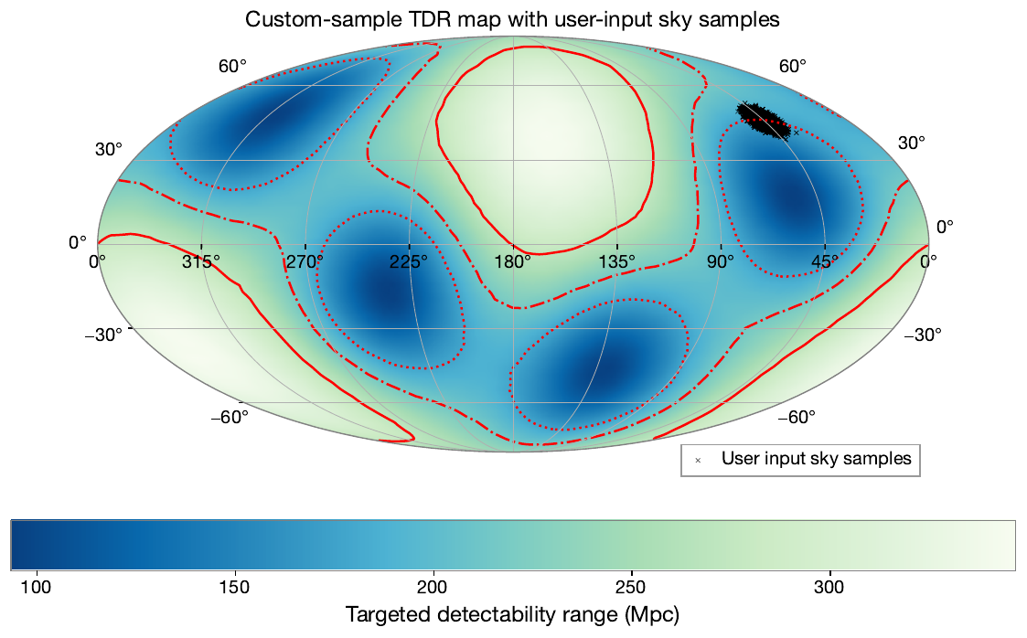
Inclination-marginalized custom-sample TDR map: /Users/samueleronchini/.cache/gw_tdr_tutorial/GRB200228A/custom_joint_tdr/range_map_bns_m1_1.4_m2_1.4.pdf
# Edit the masses (solar masses) and inclination interval (degrees) before running.
CUSTOM_M1 = 2.0
CUSTOM_M2 = 1.3
CUSTOM_IOTA_MIN_DEG = 10.0
CUSTOM_IOTA_MAX_DEG = 85.0

if not (np.isfinite(CUSTOM_M1) and np.isfinite(CUSTOM_M2) and 0 < CUSTOM_M2 <= CUSTOM_M1):
    raise ValueError('Masses must be finite and satisfy 0 < CUSTOM_M2 <= CUSTOM_M1.')
if not (np.isfinite(CUSTOM_IOTA_MIN_DEG) and np.isfinite(CUSTOM_IOTA_MAX_DEG)
        and 0 <= CUSTOM_IOTA_MIN_DEG < CUSTOM_IOTA_MAX_DEG <= 90):
    raise ValueError('Choose an inclination interval with 0 <= min < max <= 90 degrees.')

# Use the requested m1=3 solar-mass boundary to select the TDR source class.
custom_cbc_type = 'nsbh' if CUSTOM_M1 > 3 else 'bns'
custom_standard_masses = CHIRP_MASSES[custom_cbc_type]
custom_standard_match = next(
    (pair for pair in custom_standard_masses if pair == (CUSTOM_M1, CUSTOM_M2)),
    None,
)
if custom_standard_match is not None:
    CUSTOM_M1, CUSTOM_M2 = custom_standard_match
if custom_cbc_type == 'bns' and not (1.0 <= CUSTOM_M2 <= CUSTOM_M1 <= 2.0):
    raise ValueError('The TDR BNS model supports component masses from 1 to 2 solar masses.')
if custom_cbc_type == 'nsbh' and (CUSTOM_M1, CUSTOM_M2) not in custom_standard_masses:
    raise ValueError(f'The TDR NSBH model supports these configured mass pairs: {custom_standard_masses}.')

custom_iota_label = f'{CUSTOM_IOTA_MIN_DEG:g}-{CUSTOM_IOTA_MAX_DEG:g}'
custom_iota_ranges = [{
    'label': custom_iota_label,
    'iota_min': np.deg2rad(CUSTOM_IOTA_MIN_DEG),
    'iota_max': np.deg2rad(CUSTOM_IOTA_MAX_DEG),
}]
custom_ifo_tag = '-'.join(online_ifos)
custom_tdr_dir = OUTPUT_ROOT / (
    f'custom_tdr_t0_{float(T0):.4f}_ifos_{custom_ifo_tag}_'
    f'm1_{CUSTOM_M1:g}_m2_{CUSTOM_M2:g}_iota_{custom_iota_label}'
)
(custom_tdr_dir / 'results').mkdir(parents=True, exist_ok=True)

# Reuse this run's PSDs; TDR creates the injections and evaluates the TDR below.
for custom_ifo in online_ifos:
    custom_psd = RUN_DIR / f'{custom_ifo.lower()}_psd.txt'
    if not custom_psd.is_file():
        raise FileNotFoundError(f'TDR PSD not found: {custom_psd}')
    shutil.copy2(custom_psd, custom_tdr_dir / custom_psd.name)

# Stage the three standard references for this class so TDR plots them with the custom system.
custom_reference_eos = ['SFHo', 'DD2'] if custom_cbc_type == 'nsbh' else [None]
for standard_m1, standard_m2 in custom_standard_masses:
    for standard_eos in custom_reference_eos:
        standard_eos_tag = f'_{standard_eos}' if standard_eos is not None else ''
        standard_filename = (
            f'results_{custom_cbc_type}{standard_eos_tag}_'
            f'm1_{standard_m1}_m2_{standard_m2}.hdf'
        )
        standard_source = RUN_DIR / 'results' / standard_filename
        standard_target = custom_tdr_dir / 'results' / standard_filename
        if not standard_source.is_file():
            raise FileNotFoundError(f'Standard TDR reference not found: {standard_source}')
        if (standard_m1, standard_m2) != (CUSTOM_M1, CUSTOM_M2):
            shutil.copy2(standard_source, standard_target)

from targ_ac_git.targ_range_snr_mf import run_pycbc_optimal_snr

custom_eos_values = ['SFHo', 'DD2'] if custom_cbc_type == 'nsbh' else [None]
for custom_eos in custom_eos_values:
    custom_eos_tag = f'_{custom_eos}' if custom_eos is not None else ''
    custom_result_file = custom_tdr_dir / 'results' / (
        f'results_{custom_cbc_type}{custom_eos_tag}_m1_{CUSTOM_M1}_m2_{CUSTOM_M2}.hdf'
    )
    if not custom_result_file.is_file():
        tdr_aux.inject(
            custom_cbc_type, T0, [ra_best, dec_best],
            CUSTOM_M1, CUSTOM_M2, 0, str(custom_tdr_dir),
            eos=custom_eos or 'SFHo',
        )
        custom_injection_file = custom_tdr_dir / 'inj' / (
            f'injections_{custom_cbc_type}{custom_eos_tag}_m1_{CUSTOM_M1}_m2_{CUSTOM_M2}.hdf'
        )
        run_pycbc_optimal_snr(
            str(custom_injection_file), str(custom_result_file),
            online_ifos, str(custom_tdr_dir),
        )

# Keep the custom curve at index 1 so it has a distinct production-plot color.
custom_plot_masses = list(custom_standard_masses)
if custom_standard_match is None:
    custom_plot_masses.insert(1, (CUSTOM_M1, CUSTOM_M2))

np.random.seed(12345 + int(round(T0)))
selected_snrs = 'matched_filter' if SNR_STATISTIC == 'mf' else 'optimal'
custom_mass_label = f'm1={CUSTOM_M1}, m2={CUSTOM_M2}'
tdr_plot = tdr_aux.pp.plot
tdr_add_legend = tdr_aux._add_tdr_legend

def plot_custom_mass_dashed(*args, **kwargs):
    if kwargs.get('label') == custom_mass_label:
        kwargs['linestyle'] = '--'
    return tdr_plot(*args, **kwargs)

def add_custom_mass_dashed_legend(masses_list, iota_ranges):
    tdr_add_legend(masses_list, iota_ranges)
    custom_index = masses_list.index((CUSTOM_M1, CUSTOM_M2))
    legend = tdr_aux.pp.gca().get_legend()
    if legend is not None:
        legend.get_lines()[custom_index].set_linestyle('--')

try:
    tdr_aux.pp.plot = plot_custom_mass_dashed
    tdr_aux._add_tdr_legend = add_custom_mass_dashed_legend
    tdr_aux.compute_range(
        ra_samples,
        dec_samples,
        online_ifos,
        {custom_cbc_type: custom_plot_masses},
        str(custom_tdr_dir),
        custom_iota_ranges,
        SNR_THRESHOLD,
        selected_snrs,
    )
finally:
    tdr_aux.pp.plot = tdr_plot
    tdr_aux._add_tdr_legend = tdr_add_legend

# Display the D90 value written by TDR and its production efficiency plot.
custom_result_json = custom_tdr_dir / f'results_{custom_cbc_type}.json'
custom_result_payload = json.loads(custom_result_json.read_text())
custom_result = custom_result_payload[custom_cbc_type][custom_mass_label]
custom_tdr_value = custom_result['tdr'][custom_iota_label]
display(pd.DataFrame([{
    'Source class': custom_cbc_type.upper(),
    'Mass pair [M_sun]': f'm1={CUSTOM_M1:g}, m2={CUSTOM_M2:g}',
    'Inclination prior [deg]': custom_iota_label,
    'IFO network': ','.join(custom_result.get('online_ifos', [])),
    'SNR statistic': custom_result.get('snr_type', selected_snrs),
    'Threshold': custom_result.get('snr_threshold', SNR_THRESHOLD),
    'D90 [Mpc]': custom_tdr_value['D90_Mpc'],
}]))
show_pdf(custom_tdr_dir / f'{custom_cbc_type}_targeted_range.pdf')
print('TDR results saved under', custom_tdr_dir)
| Source class | Mass pair [M_sun] | Inclination prior [deg] | IFO network | SNR statistic | Threshold | D90 [Mpc] | |
|---|---|---|---|---|---|---|---|
| 0 | BNS | m1=2, m2=1.3 | 10-85 | H1,L1,V1 | matched_filter | 8.5 | 134.299118 |
TDR results saved under /Users/samueleronchini/.cache/gw_tdr_tutorial/GRB200228A/custom_tdr_t0_1266908331.0000_ifos_H1-L1-V1_m1_2_m2_1.3_iota_10-85
Run TDR from the command line#
From the repository root, with the TDR Python environment active, run either example below. Inclination limits and sky coordinates are in degrees. Use either a fixed --ra/--dec position or a HEALPix --skymap-file (not both). Replace the output directory if you have already run an example there.
Fixed sky position:
python -m targ_ac_git.targ_range_snr_mf \
  --grb-name GRB200228A_point \
  --t0 '2020-02-28T06:58:33.806' \
  --output-dir tdr/GRB200228A_point_cli \
  --ra 333.89292 --dec -42.944167 \
  --iota-min 10 --iota-max 85 \
  --snr-threshold 8.5 --snr-type mf
HEALPix sky map:
python -m targ_ac_git.targ_range_snr_mf \
  --grb-name GRB200228A_skymap \
  --t0 '2020-02-28T06:58:33.806' \
  --output-dir tdr/GRB200228A_skymap_cli \
  --skymap-file tdr/glg_healpix_all_bn200228291_v00.fit \
  --iota-min 10 --iota-max 85 \
  --snr-threshold 8.5 --snr-type mf
The inclination range is sampled as an isotropic prior truncated to those bounds. The CLI also evaluates the standard 0–90° prior for comparison. Outputs, including result JSON and plots, are written under the selected output directory.