
Tutorial 1: Top-Hat Jet Model (Flat \(\theta_c\) Distribution)#
This tutorial demonstrates the flat top-hat model, the simplest jet geometry in the MAGGPY framework. We will:
Define the prior and parameter space
Explain the \(\theta_c\) distribution and geometric efficiencies
Run a short MCMC
Visualize the resulting CDFs
Fix a median viewing angle and extract the \(f_j\) posterior
The Flat Top-Hat Model#
In the top-hat model, the GRB jet has a uniform luminosity profile within the core angle \(\theta_c\) and zero emission outside. The key simplification compared to the structured jet model is that there is no time evolution, we sample the luminosity directly.
The opening angle \(\theta_c\) is drawn from a flat (uniform) distribution between \(\theta_{c,\min} = 1°\) and \(\theta_{c,\max}\) (a free parameter).
Import Libraries#
%load_ext autoreload
%autoreload 2
import notebook_setup

import  src.init
import  emcee
import  corner
import  numpy                   as np
import  matplotlib.pyplot       as plt
from    math                    import inf
from    pathlib                 import Path

# Top-hat jet model specific modules
from    src.top_hat.montecarlo  import *
from    src.top_hat.plot        import TopHatPlotter
from    src.top_hat.geometric_eff import geometric_efficiency_flat

# Apply custom plotting style
# plt.style.use('../configurations/style.mplstyle') if you have latex
# conda install -n acme_env -c conda-forge texlive-core dvipng cm-super if you want to use the latex style, otherwise use the default matplotlib style or a custom one without latex support.
Key Ingredients: The Physics Behind the Model#
Before we set up the MCMC, let’s walk through the key physical ingredients one by one.
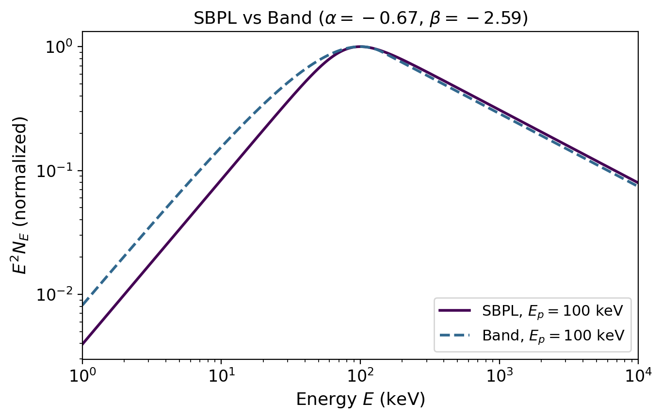
The Smoothly Broken Power Law (SBPL) Spectrum#
The photon spectrum of each GRB follows a smoothly broken power law:
where:
\(\alpha = -0.67\) is the low-energy spectral index (close to the synchrotron prediction \(\alpha = -2/3\))
\(\beta = -2.59\) is the high-energy spectral index
\(n = 2\) controls the smoothness of the break between the two power laws
\(E_j = E_p / \epsilon\) is the break energy, related to the peak energy \(E_p\)
\(C_n = 2^{1/n}\) is a normalisation constant
The peak of \(E^2 N_E\) (the \(\nu F_\nu\) spectrum) occurs at \(E_p\). This is the quantity we compare to Fermi-GBM observations.
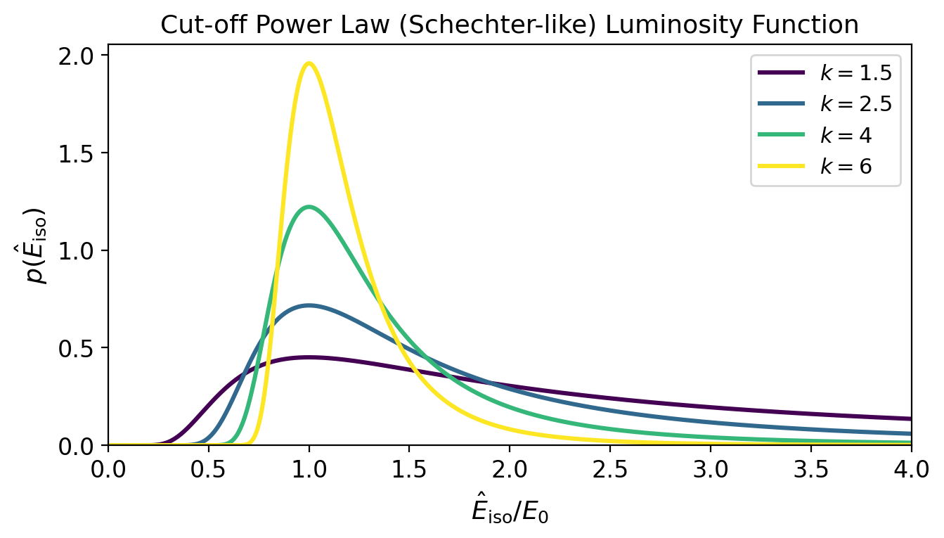
The Cut-off Power Law (Luminosity Function)#
The isotropic-equivalent energy \(\hat{E}_{\rm iso}\) of each GRB is drawn from a cut-off power law (Schechter-like function):
The parameter \(k\) controls the shape:
Small \(k\) (\(\sim 1.5\)): broad distribution, many high-energy events
Large \(k\) (\(\gtrsim 4\)): steep drop-off, most events are low-energy
\(E_0\) (parametrised as L_L0 \(= \log_{10}(E_0 / 10^{49}\,\text{erg/s})\)) sets the overall energy scale.
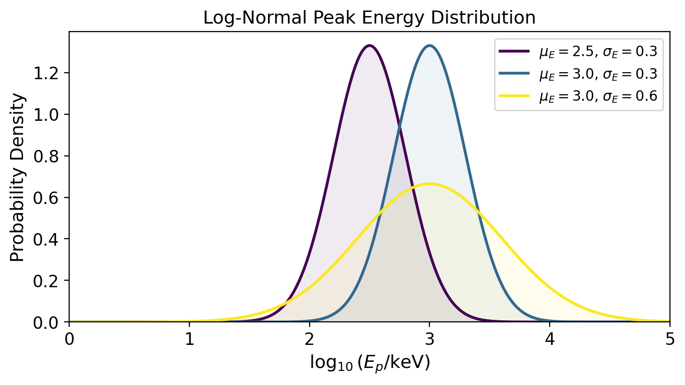
Peak Energy Distribution (\(E_p\))#
The rest-frame peak energy \(E_{p,\text{rest}}\) is drawn from a log-normal distribution:
L_mu_E\(= \log_{10}(\mu_E / \text{keV})\): the mean of the distribution (typically \(\sim 10^{2.5}\)–\(10^{3.5}\) keV)sigma_E: the width (scatter) of the distribution in log-space
The observed peak energy is redshifted: \(E_{p,\text{obs}} = E_{p,\text{rest}} / (1+z)\).
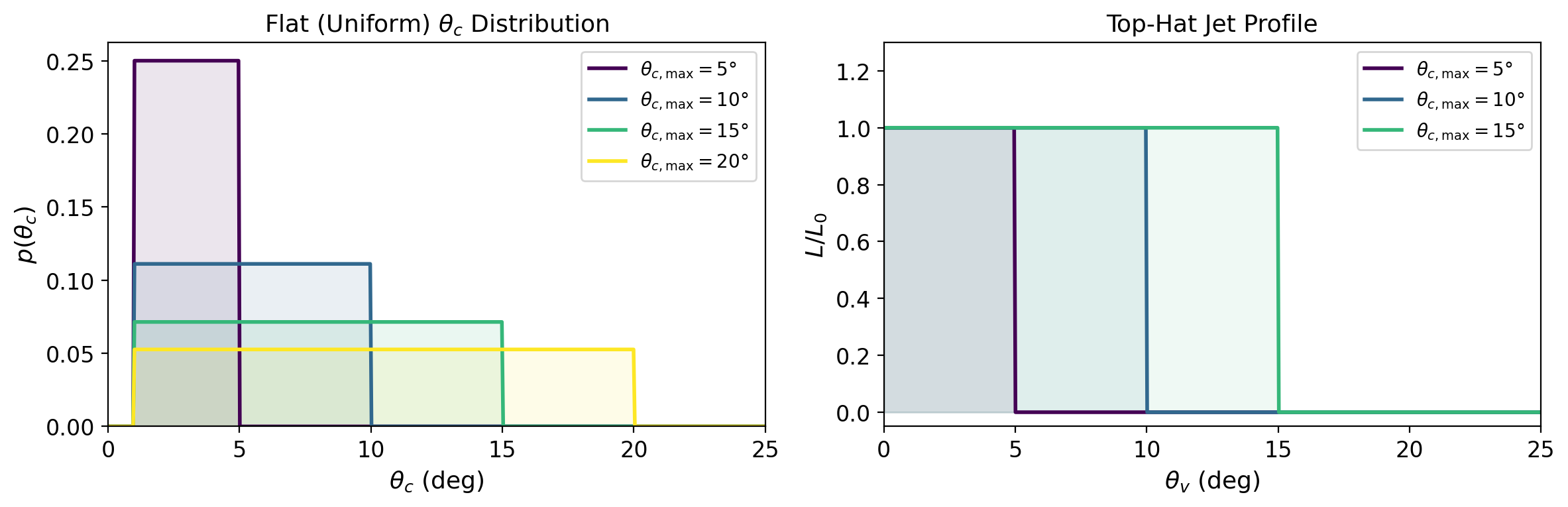
The Top-Hat \(\theta_c\) Distribution#
In the top-hat model, every jet has a uniform luminosity profile: full brightness for \(\theta_v \leq \theta_c\), and zero outside. The core angle \(\theta_c\) is not fixed but drawn from a flat (uniform) distribution between:
This means:
All angles from 1° to \(\theta_{c,\max}\) are equally likely
The only free parameter for the geometry is \(\theta_{c,\max}\)
A larger \(\theta_{c,\max}\) means wider jets are possible → more detectable GRBs
The figure below shows this flat window and the resulting jet profile:
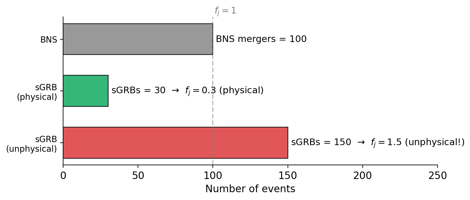
The Jet Fraction \(f_j\)#
The jet fraction is defined as the ratio of short GRBs to BNS mergers:
Its physical meaning:
\(f_j \leq 1\) (physical): not every BNS merger produces a detectable sGRB. Some mergers might not launch a jet, or the jet may be too weak. \(f_j = 0.3\) means only 30% of BNS mergers produce an observable sGRB.
\(f_j = 1\): every BNS merger produces exactly one sGRB.
\(f_j > 1\) (unphysical): there would be more sGRBs than BNS mergers, which is not possible if BNS mergers are the sole progenitor. Values \(f_j > 1\) returned by the MCMC indicate the model is trying to overcompensate for low detection efficiency and may signal model tension.
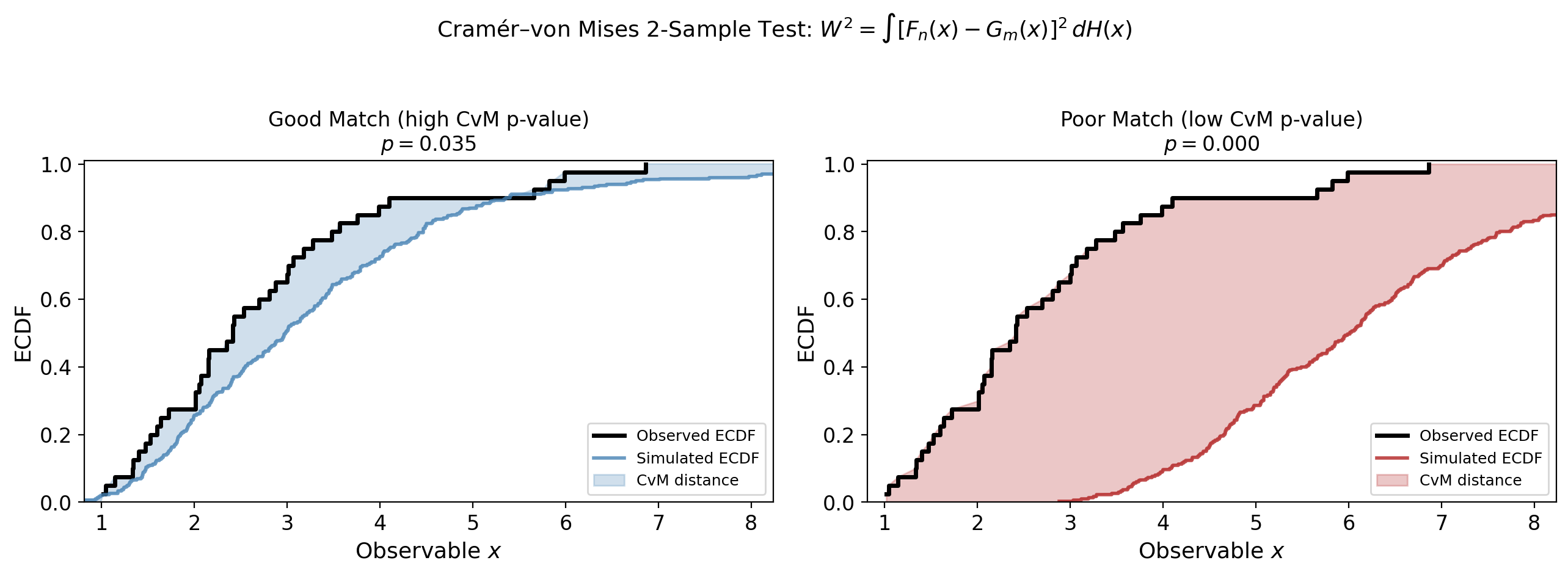
The Cramér–von Mises (CvM) Goodness-of-Fit Test#
We need a way to measure how well the simulated GRB observables match the real Fermi-GBM data. We use the Cramér–von Mises 2-sample test.
Definition#
Given two samples \(\{x_1, \dots, x_n\}\) (observed) and \(\{y_1, \dots, y_m\}\) (simulated), the CvM statistic measures the integrated squared distance between their empirical CDFs:
where \(F_n\) and \(G_m\) are the empirical CDFs of the two samples and \(H_{n+m}\) is the CDF of the pooled sample.
How we use it#
The test returns a p-value: high \(p\) means the two distributions are consistent; low \(p\) means they differ.
We compute CvM tests in \(\log_{10}\)-space for both peak flux (\(F_p\)) and peak energy (\(E_p\)).
The shape log-likelihood is: \(\ln \mathcal{L}_{\rm shape} = \ln p_{\rm CvM}(F_p) + \ln p_{\rm CvM}(E_p)\)
The image below illustrates the idea — the shaded area between the two ECDFs is what the CvM statistic captures:
Setup#
datafiles   = Path("../datafiles")
N_WALKERS   = 20
1. Parameters and Priors#
The flat top-hat model has 6 free parameters (see the explanations in the section above for physical details):
Parameter |
Symbol |
Description |
Prior Range |
|---|---|---|---|
|
\(k\) |
Power-law index of the cut-off power law luminosity function |
\([1.5, 12]\) |
|
\(\log_{10}(L_0/10^{49}\,\text{erg/s})\) |
Isotropic energy scale |
\([-2, 7]\) |
|
\(\log_{10}(\mu_E/\text{keV})\) |
Mean of the log-normal peak energy distribution |
\([0.1, 7]\) |
|
\(\sigma_E\) |
Width of peak energy log-normal distribution (in dex) |
\([0, 2.5]\) |
|
\(\theta_{c,\max}\) |
Upper bound of the uniform \(\theta_c\) window (deg) |
\([1, 25]\) |
|
\(f_j = N_{\rm sGRB}/N_{\rm BNS}\) |
Jet fraction (\(\leq 1\) physical, \(>1\) unphysical) |
\([0, 10]\) |
We use flat (uniform) priors for all parameters.
N_PARAMS    = 6
PARAM_NAMES = ["A_index", "L_L0", "L_mu_E", "sigma_E", "theta_c_max", "fj"]

def log_prior_flat_tophat(thetas):
    """Flat (uniform) prior for the top-hat model."""
    A_index, L_L0, L_mu_E, sigma_E, theta_c_max, fj = thetas

    if not (1.5 < A_index       < 12):  return -inf
    if not (-2  < L_L0          < 7):   return -inf
    if not (0.1 < L_mu_E        < 7):   return -inf
    if not (0   < sigma_E       < 2.5): return -inf
    if not (1   < theta_c_max   < 25):  return -inf
    if not (0   < fj            < 10):   return -inf

    return 0.0

print("Prior test (valid point):",   log_prior_flat_tophat([3, 1, 3, 0.5, 10, 0.5]))
print("Prior test (invalid point):", log_prior_flat_tophat([3, 1, 3, 0.5, 30, 0.5]))
Prior test (valid point): 0.0
Prior test (invalid point): -inf
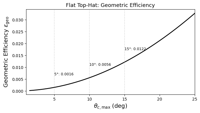
2. Geometric Efficiency#
The geometric efficiency \(\epsilon_{\text{geo}}\) is the probability that a randomly oriented observer falls within the jet cone. Let’s derive it from scratch.
Derivation#
The viewing angle \(\theta_v\) (angle between the jet axis and the line of sight) is distributed as:
This is because isotropically distributed orientations yield a \(\sin\theta_v\) probability density on the sphere (the fraction of solid angle at angle \(\theta_v\) is \(\propto \sin\theta_v\)).
For a top-hat jet with opening angle \(\theta_c\), we detect the GRB only if \(\theta_v \leq \theta_c\). The geometric efficiency for a fixed \(\theta_c\) is therefore:
Example: for \(\theta_c = 3.4° \approx 0.059\) rad, \(\epsilon_{\rm geo} = 1 - \cos(3.4°) \approx 1.8 \times 10^{-3}\) — only ~0.2% of orientations fall within the cone!
Averaging over a flat \(\theta_c\) distribution#
In our model, \(\theta_c\) is not fixed but drawn from \(\text{Uniform}(\theta_{c,\min}, \theta_{c,\max})\). The average geometric efficiency is:
This is a key quantity because the total detection efficiency is: $\( \epsilon = \epsilon_{\text{geo}} \times f_j \times \epsilon_{\text{GBM}} \)$
Let’s visualize how \(\epsilon_{\text{geo}}\) varies with \(\theta_{c,\max}\):
theta_max_arr = np.linspace(1.5, 25, 200)
geo_eff_arr   = [geometric_efficiency_flat(t) for t in theta_max_arr]

fig, ax = plt.subplots(figsize=(7, 4))
ax.plot(theta_max_arr, geo_eff_arr, 'k-', lw=2)
ax.set_xlabel(r'$\theta_{c,\max}$ (deg)', fontsize=14)
ax.set_ylabel(r'Geometric Efficiency $\epsilon_{\text{geo}}$', fontsize=14)
ax.set_title('Flat Top-Hat: Geometric Efficiency', fontsize=13)

# Mark some reference values
for t_ref in [5, 10, 15]:
    eff = geometric_efficiency_flat(t_ref)
    ax.axvline(t_ref, ls=':', alpha=0.4, color='grey')
    ax.annotate(f'{t_ref}°: {eff:.4f}', xy=(t_ref, eff), fontsize=9,
                xytext=(t_ref+0.01, eff + 0.005))

ax.set_xlim(1, 25)
plt.tight_layout()
plt.show()
3. Likelihood and Walker Initialization#
The likelihood combines shape and rate terms (see the CvM explanation above):
Monte Carlo generation: draw \(\hat{E}_{\rm iso}\) from the cut-off power law, \(E_p\) from the log-normal, assign random redshifts and \(\theta_c\) values from the flat distribution.
Detection cuts: keep events with \(F_p > 4\,\text{ph}/\text{cm}^2/\text{s}\) and \(E_p \in [50, 10\,000]\,\text{keV}\).
Shape likelihood: CvM test on \(F_p\) and \(E_p\) distributions \(\to \ln \mathcal{L}_{\rm shape}\).
Rate likelihood: Poisson probability of observing \(N_{\rm obs}\) given \(N_{\rm pred}\) \(\to \ln \mathcal{L}_{\rm rate}\).
def log_likelihood_flat_tophat(thetas, params_in, distances, k_interpolator, n_events=10_000):
    """Log-likelihood for the flat top-hat model."""
    theta_c_max, fj = thetas[4], thetas[5]

    gbm_eff              = 0.6
    geometric_efficiency = geometric_efficiency_flat(theta_c_max)
    triggered_years      = params_in.triggered_years
    epsilon              = geometric_efficiency * fj

    n_years              = triggered_years
    intrinsic_rate       = epsilon * len(params_in.z_arr) * gbm_eff
    expected_events      = intrinsic_rate * n_years

    # Run the simplified Monte Carlo
    results = simplified_montecarlo(thetas, n_events, params_in, distances, k_interpolator)

    # Apply detection cuts
    trigger_mask, analysis_mask = apply_detection_cuts(results["p_flux"], results["E_p_obs"])

    if np.sum(analysis_mask) <= 3:
        return -inf, -inf, -inf, -inf, -inf

    triggered_events    = np.sum(trigger_mask)
    physics_efficiency  = triggered_events / n_events
    predicted_detections = expected_events * physics_efficiency
    observed_detections  = params_in.yearly_rate * params_in.triggered_years

    # Score functions
    l1 = score_func_cvm(results["p_flux"][analysis_mask], params_in.pflux_data, params_in.rng)
    l2 = score_func_cvm(results["E_p_obs"][analysis_mask], params_in.epeak_data, params_in.rng)
    l3 = poiss_log(k=observed_detections, mu=predicted_detections)

    return l1 + l2 + l3, l1, l2, l3, physics_efficiency


def initialize_walkers_flat(n_walkers):
    """Initialize walkers within the prior bounds."""
    np.random.seed(42)
    return np.column_stack([
        np.random.uniform(2, 3, n_walkers),        # A_index
        np.random.uniform(2, 4, n_walkers),        # L_L0
        np.random.uniform(2, 4, n_walkers),        # L_mu_E
        np.random.uniform(0.2, 1, n_walkers),      # sigma_E
        np.random.uniform(5, 15, n_walkers),       # theta_c_max
        np.random.uniform(0.3, 0.8, n_walkers),    # fj
    ])

print(f"Example initial walker: {initialize_walkers_flat(1)[0]}")
Example initial walker: [2.37454012 3.90142861 3.46398788 0.67892679 6.5601864 0.37799726]
4. Initialize the Simulation and Run MCMC#
# Initialize simulation (loads GBM data, creates interpolators)
params = {
    "alpha"       : -0.67,
    "beta_s"      : -2.59,
    "n"           : 2,
    "theta_c"     : 3.4,
    "theta_v_max" : 10,
    "z_model"     : 'fiducial_Hrad_TEST_A1.0'  # Change to 'fiducial_Hrad_TEST_A1.0' to use Tutorial 0 samples
}

default_params, _, data_dict = src.init.initialize_simulation(datafiles, params=params)
print(f"Catalogue events: {len(default_params.pflux_data)}")
print(f"Yearly rate: {default_params.yearly_rate:.1f} GRBs/yr")
print(f"Triggered years: {default_params.triggered_years:.1f}")
Using redshift model: samples_fiducial_Hrad_TEST_A1.0.dat with 360832 BNSs.
Warning: Could not load MRD distribution: MRD file not found: ../datafiles/populations/MRD/output_sigma0.1/fiducial_Hrad_TEST/A1.0/BNSs/MRD_spread_15Z_40_No_MandF2017_0.1_No_No_0.dat
Continuing without P(z) interpolator.
Defaulting to values for Fiducial populations
Generating temporal interpolators... (this may take a moment)
Preparing catalogue with limits: {'F_LIM': 4, 'T90_LIM': 2, 'EP_LIM_UPPER': 10000, 'EP_LIM_LOWER': 50}
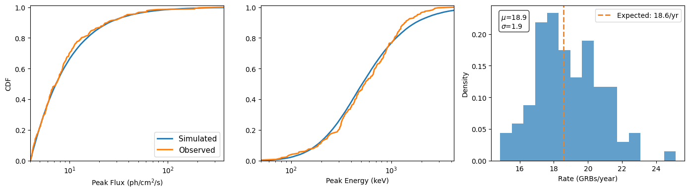
Triggered events: 325, Trigger years: 17.50, Yearly rate: 18.58 events/year
Catalogue events: 268
Yearly rate: 18.6 GRBs/yr
Triggered years: 17.5
# Create output directory and configure MCMC
output_dir  = src.init.create_run_dir("tutorial1_tophat_flat")

n_walkers   = 20
n_steps     = 2000  # Use more steps (e.g. 50 000) for production runs

# Create the k-factor interpolator (redshift correction)
k_interpolator = create_k_interpolator()

# Build the log-probability function
log_probability_flat = create_log_probability_function(
    log_prior_func      = log_prior_flat_tophat,
    log_likelihood_func  = log_likelihood_flat_tophat,
    params_in            = default_params,
    k_interpolator       = k_interpolator
)

# Check for existing chain or start fresh
initial_pos, n_steps_remaining, backend = check_and_resume_mcmc(
    filename                = output_dir / "emcee.h5",
    n_steps                 = n_steps,
    initialize_walkers_func = initialize_walkers_flat,
    n_walkers               = n_walkers
)

# Run the MCMC
if n_steps_remaining > 0:
    sampler = run_mcmc(
        log_probability_func = log_probability_flat,
        initial_walkers      = initial_pos,
        n_iterations         = n_steps_remaining,
        n_walkers            = n_walkers,
        n_params             = N_PARAMS,
        backend              = backend,
    )
else:
    print("MCMC already complete, loading results.")
Creating new directory : Output_files/tutorial1_tophat_flat
Starting new run
100%|██████████| 2000/2000 [00:46<00:00, 42.57it/s]
5. Results: CDFs and Diagnostics#
The TopHatPlotter provides all the standard diagnostic plots.
backend_flat = emcee.backends.HDFBackend(output_dir / "emcee.h5")
BURN_IN = 200

plotter = TopHatPlotter(
    backend     = backend_flat,
    output_dir  = output_dir,
    model_type  = "flat_theta",
    burn_in     = BURN_IN,
    thin        = 10
)
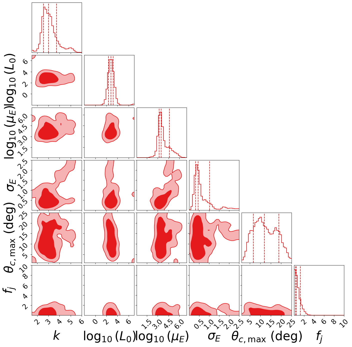
Corner Plot#
plotter.plot_corner(filename="corner_flat_tophat.pdf")
(3600, 6)
CDF Comparison#
Compare the simulated peak flux and peak energy CDFs against the observed Fermi-GBM data.
distances = compute_luminosity_distance(default_params.z_arr)

plotter.plot_cdf_comparison(
    mc_func          = simplified_montecarlo,
    params_in        = default_params,
    distances        = distances,
    k_interpolator   = k_interpolator,
    geometric_eff_func = geometric_efficiency_flat,
    n_samples        = 100,
    filename         = "cdf_flat_tophat.pdf"
)
Summary Table#
print(plotter.summary_table())
\begin{tabular}{lc}
\hline
Parameter & Value \\
\hline
$k$ & $3.008_{-0.462}^{+0.715}$ \\
$\log_{10}(L_0)$ & $2.811_{-0.444}^{+0.421}$ \\
$\log_{10}(\mu_E)$ & $3.480_{-0.267}^{+1.136}$ \\
$\sigma_E$ & $0.455_{-0.128}^{+0.572}$ \\
$\theta_{c,\max}$ (deg) & $11.895_{-5.241}^{+7.007}$ \\
$f_j$ & $0.463_{-0.218}^{+0.791}$ \\
\hline
\end{tabular}
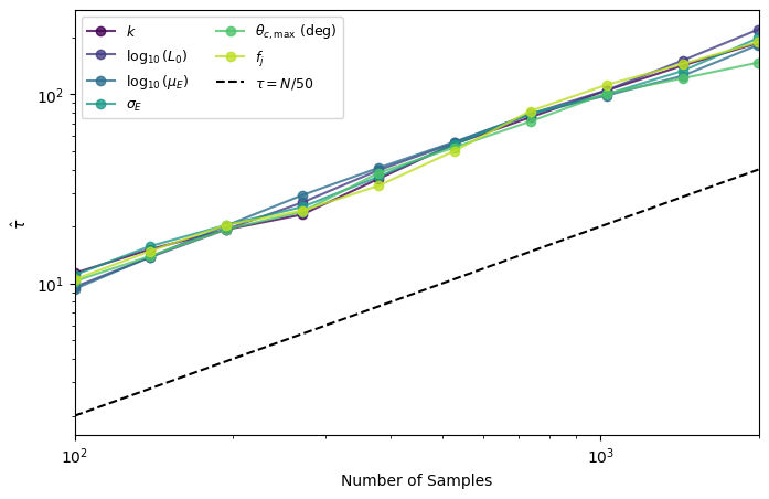
Autocorrelation#
plotter.plot_autocorrelation()
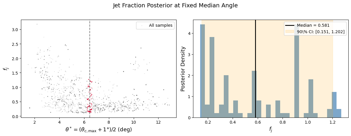
6. Extracting the \(f_j\) Posterior at a Fixed Viewing Angle#
A useful exercise is to fix the median opening angle and study how the jet fraction \(f_j\) is constrained. We choose \(\theta^* = (\theta_{c,\max} + 1°) / 2\), which is the median of the flat \(\theta_c\) distribution.
Procedure:#
Extract full posterior samples
Compute \(\theta^* = (\theta_{c,\max} + 1) / 2\) for each sample
Slice the \(f_j\) posterior at a given fixed \(\theta^*\)
# Get the full posterior samples
samples = backend_flat.get_chain(discard=BURN_IN, thin=10, flat=True)

theta_c_max_samples = samples[:, 4]  # theta_c_max
fj_samples          = samples[:, 5]  # fj

# Compute the median angle for each sample: theta* = (theta_c_max + 1) / 2
theta_star = (theta_c_max_samples + 1) / 2

print(f"theta* range: [{theta_star.min():.1f}, {theta_star.max():.1f}] deg")
print(f"theta* median: {np.median(theta_star):.1f} deg")
print(f"fj median: {np.median(fj_samples):.3f}")
theta* range: [1.5, 12.9] deg
theta* median: 6.4 deg
fj median: 0.463
# Fix theta* at a specific value and look at fj conditioned on that
# We select samples where theta* is close to a target value
target_theta_star = np.median(theta_star)
tolerance         = 0.2  # degrees

mask = np.abs(theta_star - target_theta_star) < tolerance
fj_conditional = fj_samples[mask]

print(f"Conditioning on θ* = {target_theta_star:.1f}° ± {tolerance}°")
print(f"Selected {np.sum(mask)} / {len(mask)} samples")

fig, (ax1, ax2) = plt.subplots(1, 2, figsize=(12, 4.5))

# Left: 2D scatter of theta* vs fj
ax1.scatter(theta_star, fj_samples, s=1, alpha=0.15, color='grey', label='All samples')
ax1.scatter(theta_star[mask], fj_samples[mask], s=2, alpha=0.4, color='crimson')
ax1.axvline(target_theta_star, ls='--', color='k', alpha=0.5)
ax1.set_xlabel(r'$\theta^* = (\theta_{c,\max} + 1°) / 2$ (deg)', fontsize=13)
ax1.set_ylabel(r'$f_j$', fontsize=13)
ax1.legend(fontsize=10)

# Right: fj posterior conditioned on theta*
lo, med, hi = np.percentile(fj_conditional, [5, 50, 95])
ax2.hist(fj_conditional, bins=30, density=True, alpha=0.7, color='steelblue')
ax2.axvline(med, ls='-', color='k', lw=2, label=f'Median = {med:.3f}')
ax2.axvspan(lo, hi, alpha=0.15, color='orange', label=f'90\% CI: [{lo:.3f}, {hi:.3f}]')
ax2.set_xlabel(r'$f_j$', fontsize=13)
ax2.set_ylabel('Posterior Density', fontsize=13)
ax2.legend(fontsize=10)

plt.suptitle('Jet Fraction Posterior at Fixed Median Angle', fontsize=14, y=1.02)
plt.tight_layout()
plt.savefig(output_dir / "fj_posterior_fixed_theta.pdf", dpi=300, bbox_inches='tight')
plt.show()
Conditioning on θ* = 6.4° ± 0.2°
Selected 132 / 3600 samples
Summary#
In this tutorial we demonstrated:
Prior definition — flat priors on 6 parameters for the top-hat model
Geometric efficiency — how \(\epsilon_{\text{geo}}(\theta_{c,\max})\) is computed for a uniform \(\theta_c\) distribution
MCMC — setting up and running
emceewith the top-hat likelihoodCDF comparison — posterior predictive checks against Fermi-GBM data
Conditional \(f_j\) posterior — fixing \(\theta^* = (\theta_{c,\max} + 1°)/2\) and extracting the jet fraction
Next: Tutorial 2 covers the full structured jet model with time evolution and richer diagnostics.
🏋️ Exercise: Universal (Fixed) Opening Angle Model#
In this exercise you will replace the flat \(\theta_c\) distribution with a universal opening angle — all BNS mergers produce jets with the same \(\theta_c\). The skeleton code is provided — fill in the missing pieces marked with ???.
Background#
In the main tutorial, \(\theta_c\) was drawn from a flat distribution between 1° and \(\theta_{c,\max}\). A simpler alternative is to assume that all BNS mergers produce jets with exactly the same opening angle \(\theta_c\):
This is the universal (or fixed) opening angle model. It has a major simplification: the geometric efficiency becomes a simple closed-form expression (recall the derivation above):
No averaging over \(\theta_c\) is needed because every jet has the same angle.
Your task: replace theta_c_max with theta_c_fixed in the prior and likelihood, and use the simplified geometric efficiency.
Step 1: Define the prior for the fixed-angle model#
The parameter theta_c_max is replaced by theta_c_fixed (the single universal opening angle, in degrees).
N_PARAMS_EX  = 6
PARAM_NAMES_EX = ["A_index", "L_L0", "L_mu_E", "sigma_E", "theta_c_fixed", "fj"]

def log_prior_fixed_angle(thetas):
    """Flat prior for the universal (fixed) opening-angle model."""
    A_index, L_L0, L_mu_E, sigma_E, theta_c_fixed, fj = thetas

    if not (1.5 < A_index       < 12):  return -inf
    if not (-2  < L_L0          < 7):   return -inf
    if not (0.1 < L_mu_E        < 7):   return -inf
    if not (0   < sigma_E       < 2.5): return -inf
    # -------------------------------------------------------
    # ✏️ EXERCISE: Add the prior bound for theta_c_fixed (in degrees).
    # What is a reasonable range? (Hint: between ~1° and ~25°)
    # -------------------------------------------------------
    if not (??? < theta_c_fixed < ???): return -inf   # <-- FIX THIS
    if not (0   < fj            < 10):  return -inf

    return 0.0

# Test
# print(log_prior_fixed_angle([3, 1, 3, 0.5, 5.0, 0.5]))
  Cell In[17], line 16
    if not (??? < theta_c_fixed < ???): return -inf   # <-- FIX THIS
            ^
SyntaxError: invalid syntax
Step 2: Modify the likelihood to use the fixed-angle geometric efficiency#
The key change: replace geometric_efficiency_flat(theta_c_max) with the simple \(1 - \cos\theta_c^*\) formula.
def log_likelihood_fixed_angle(thetas, params_in, distances, k_interpolator, n_events=10_000):
    """Log-likelihood for the top-hat model with a FIXED (universal) opening angle."""
    theta_c_fixed = thetas[4]   # single angle in degrees
    fj            = thetas[5]

    gbm_eff          = 0.6
    triggered_years  = params_in.triggered_years

    # -------------------------------------------------------
    # ✏️ EXERCISE: Compute the geometric efficiency for a fixed angle.
    # Recall: epsilon_geo = 1 - cos(theta_c)  (theta_c in RADIANS!)
    # Hint: geometric_efficiency = 1 - np.cos(np.deg2rad(???))
    # -------------------------------------------------------
    geometric_efficiency = ???   # <-- FIX THIS

    epsilon          = geometric_efficiency * fj
    n_years          = triggered_years
    intrinsic_rate   = epsilon * len(params_in.z_arr) * gbm_eff
    expected_events  = intrinsic_rate * n_years

    # Run the Monte Carlo (the spectral part is unchanged — thetas[:4] are the same)
    results = simplified_montecarlo(thetas, n_events, params_in, distances, k_interpolator)

    # Apply detection cuts (unchanged)
    trigger_mask, analysis_mask = apply_detection_cuts(results["p_flux"], results["E_p_obs"])

    if np.sum(analysis_mask) <= 3:
        return -inf, -inf, -inf, -inf, -inf

    triggered_events     = np.sum(trigger_mask)
    physics_efficiency   = triggered_events / n_events
    predicted_detections = expected_events * physics_efficiency
    observed_detections  = params_in.yearly_rate * params_in.triggered_years

    # Score functions (unchanged)
    l1 = score_func_cvm(results["p_flux"][analysis_mask], params_in.pflux_data, params_in.rng)
    l2 = score_func_cvm(results["E_p_obs"][analysis_mask], params_in.epeak_data, params_in.rng)
    l3 = poiss_log(k=observed_detections, mu=predicted_detections)

    return l1 + l2 + l3, l1, l2, l3, physics_efficiency
Step 3: Initialize walkers and run a short MCMC#
Update the walker initialisation for theta_c_fixed and run a short chain.
def initialize_walkers_fixed_angle(n_walkers):
    """Initialize walkers for the fixed-angle model."""
    np.random.seed(42)
    return np.column_stack([
        np.random.uniform(2, 3, n_walkers),        # A_index
        np.random.uniform(2, 4, n_walkers),        # L_L0
        np.random.uniform(2, 4, n_walkers),        # L_mu_E
        np.random.uniform(0.2, 1, n_walkers),      # sigma_E
        # -------------------------------------------------------
        # ✏️ EXERCISE: Add initial values for theta_c_fixed (degrees)
        # Hint: np.random.uniform(???, ???, n_walkers)
        # -------------------------------------------------------
        np.random.uniform(???, ???, n_walkers),     # theta_c_fixed  <-- FIX THIS
        np.random.uniform(0.3, 0.8, n_walkers),    # fj
    ])


# -------------------------------------------------------
# ✏️ EXERCISE: Build the log-probability and run a short MCMC.
# Use create_log_probability_function with your new prior & likelihood,
# then run ~500 steps to see if the chain converges.
# -------------------------------------------------------

# output_dir_ex = src.init.create_run_dir("tutorial1_exercise_fixed_angle")
#
# log_probability_ex = create_log_probability_function(
#     log_prior_func       = log_prior_fixed_angle,
#     log_likelihood_func  = log_likelihood_fixed_angle,
#     params_in            = default_params,
#     k_interpolator       = k_interpolator
# )
#
# pos_ex = initialize_walkers_fixed_angle(20)
# backend_ex = emcee.backends.HDFBackend(output_dir_ex / "emcee.h5")
# backend_ex.reset(20, N_PARAMS_EX)
#
# sampler_ex = run_mcmc(
#     log_probability_func = log_probability_ex,
#     initial_walkers      = pos_ex,
#     n_iterations         = 500,
#     n_walkers            = 20,
#     n_params             = N_PARAMS_EX,
#     backend              = backend_ex,
# )
#
# print("Exercise MCMC complete!")
🤔 Questions to Think About#
Once you have the exercise running, consider:
Geometric efficiency: How does \(\epsilon_{\rm geo} = 1 - \cos\theta_c^*\) compare to the flat-distribution formula for typical \(\theta_c\) values? Plot both on the same axes.
Constraint on \(\theta_c^*\): How does the MCMC constrain \(\theta_c^*\) more differently than \(\theta_{c,\max}\) in the original model? Is the posterior narrower or wider? Why? (Hint: Think of the efficiency)
Physical realism: The universal model assumes every BNS merger produces a jet with exactly the same opening angle. Is this a reasonable assumption? What physical effects could cause a distribution of \(\theta_c\) values?
\(f_j\) posterior: Compare the \(f_j\) posterior between the universal and flat \(\theta_c\) models. Does the universal model prefer higher or lower \(f_j\) values? Why?
Next: Tutorial 2 covers the full structured jet model with time evolution and richer diagnostics.