
Tutorial 3: GW Detection Efficiency with GWFish#
This notebook computes the gravitational-wave detection efficiency for BNS mergers associated with short GRBs, using the GWFish Fisher-matrix package.
Setup#
We start with a two-detector Einstein Telescope network:
Label |
Detectors |
|---|---|
ET 2L network |
|
For each event in the GRB catalogue (produced in Tutorial 2), we:
Assign BNS parameters (masses, sky position, polarisation, …)
Compute the network SNR via GWFish
Apply an SNR threshold to determine detection
Derive the detection rate and its Poisson uncertainty
Exercise at the end: You will extend the network by adding Cosmic Explorer (
CE40) and compare the detection rates.
Import Libraries#
%load_ext autoreload
%autoreload 2
import notebook_setup

import multiprocessing as mp
cpus = mp.cpu_count()

import warnings
warnings.filterwarnings("ignore", "Wswiglal-redir-stdio")

import numpy             as np
import pandas            as pd
import matplotlib.pyplot as plt
import GWFish.modules    as gw
from   astropy.cosmology import Planck18
from   pathlib           import Path

#plt.style.use('../configurations/style.mplstyle')

datafiles  = Path("../datafiles")
output_dir = Path("Output_files/tutorial3_gwfish")
output_dir.mkdir(parents=True, exist_ok=True)
Background: Matched Filtering & Signal-to-Noise Ratio#
Before diving into the pipeline, let’s understand what GWFish actually computes when it returns an SNR value.
The Data Stream#
A GW detector measures a time-series of strain:
where \(h_{\boldsymbol{\theta}}(t)\) is the gravitational-wave signal (parameterised by source properties \(\boldsymbol{\theta}\)) and \(n(t)\) is detector noise. The noise has both Gaussian (thermal, quantum shot noise, seismic) and non-Gaussian (glitches, scattered light) components. For the purpose of detection, we model \(n(t)\) as a stationary Gaussian process.
Noise Characterisation: the Power Spectral Density#
The statistical properties of the noise are fully captured by the one-sided Power Spectral Density (PSD) \(S_n(f)\), defined via:
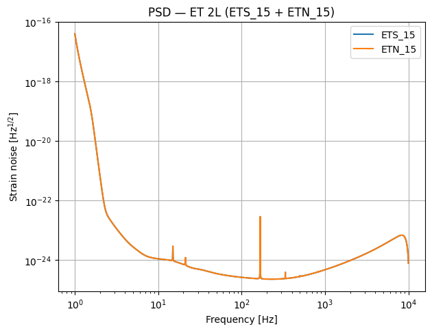
where \(\tilde{n}(f)\) is the Fourier transform of \(n(t)\). The PSD tells us the noise power per unit frequency — lower \(S_n(f)\) means better sensitivity at that frequency. When we plot the PSDs below (Step 3), you will see the characteristic “bucket” shape: seismic noise dominates at low frequencies, shot noise at high frequencies, and the best sensitivity lies in between.
The Noise-Weighted Inner Product#
To optimally distinguish a signal from noise, we define a noise-weighted inner product between two frequency-domain signals:
This is the foundation of matched filtering: frequencies where the detector is noisy (\(S_n\) large) are automatically down-weighted, while sensitive frequencies contribute more.
Optimal SNR#
The optimal signal-to-noise ratio — the quantity GWFish computes — is then:
This represents the best possible SNR achievable with a perfectly matching template. It depends on: (i) the signal amplitude \(|\tilde{h}(f)|\) (set by the source parameters), and (ii) the detector noise \(S_n(f)\) (set by the instrument).
Intuition: The integrand \(|\tilde{h}(f)|^2 / S_n(f)\) is the SNR density per frequency bin. Plotting this “weighted strain” reveals which frequencies contribute most to the detection — for BNS systems, this is typically tens to hundreds of Hz where 3G detectors are most sensitive.
Toy Example: Recovering a Signal from Noise#
To build intuition, here is a minimal matched-filtering demo. We bury a known sine-wave “signal” in Gaussian noise, then show how cross-correlating the data with the correct template recovers the signal and yields an SNR.
# --- Toy matched-filtering example ---
np.random.seed(0)
from scipy.signal import windows
from scipy.fft import fft, ifft

# Time array
fs = 1024          # sampling rate (Hz)
T  = 2.0           # duration (s)
t  = np.arange(0, T, 1/fs)
N  = len(t)

# "Signal": a chirp-like sine wave (frequency sweeps from 30 to 80 Hz)
f0, f1 = 30, 80
phase  = 2 * np.pi * (f0 * t + (f1 - f0) / (2 * T) * t**2)
signal = 1.0 * np.sin(phase) * np.exp(-((t - T/2) / 0.4)**2)  # Gaussian envelope

# "Noise": white Gaussian noise (σ = 1)
noise = np.random.normal(0, 1, N)

# "Data": signal + noise
data = signal + noise

# ---- Matched filter (detection statistic) ----
# Shift template so peak is at t=0 → MF output peaks at signal's arrival time
peak_idx = np.argmax(np.abs(signal))
template = np.roll(signal, -peak_idx)

H_templ = fft(template)
D       = fft(data)
mf_output = np.real(ifft(D * np.conj(H_templ)))
mf_output /= np.sqrt(np.sum(signal**2))  # normalise so peak ≈ SNR

# ---- Wiener filter (signal reconstruction) ----
# Recovers the signal *shape* from noisy data: W(f) = |H|^2 / (|H|^2 + σ_n^2)
H_sig    = fft(signal)
sigma2   = 1.0  # known noise variance
wiener_W = np.abs(H_sig)**2 / (np.abs(H_sig)**2 + sigma2 * N)
recovered = np.real(ifft(D * wiener_W))

# --- Plot ---
fig, axes = plt.subplots(4, 1, figsize=(10, 9), sharex=True)

axes[0].plot(t, signal, color='#31688e', lw=1.2)
axes[0].set_ylabel('Strain')
axes[0].set_title('(a) True signal (hidden chirp)', fontsize=12)
axes[0].set_ylim(-1.5, 1.5)

axes[1].plot(t, data, color='grey', lw=0.5, alpha=0.8, label='data = signal + noise')
axes[1].plot(t, signal, color='#31688e', lw=1.2, alpha=0.6, label='true signal')
axes[1].set_ylabel('Strain')
axes[1].set_title('(b) Observed data  $d(t) = h(t) + n(t)$', fontsize=12)
axes[1].legend(fontsize=9, loc='upper right')
axes[1].set_ylim(-4, 4)

axes[2].plot(t, mf_output, color='#440154', lw=1.2)
axes[2].axhline(0, ls='-', color='grey', lw=0.5)
peak_snr = mf_output.max()
peak_time = t[np.argmax(mf_output)]
axes[2].axhline(peak_snr, ls='--', color='#e15759', lw=1,
                label=rf'peak SNR $\approx {peak_snr:.1f}$ at $t = {peak_time:.2f}$ s')
axes[2].set_ylabel('SNR')
axes[2].set_title('(c) Matched-filter output — detection statistic (finds *when*)', fontsize=12)
axes[2].legend(fontsize=9, loc='upper right')

axes[3].plot(t, signal, color='#31688e', lw=1.2, alpha=0.4, label='true signal')
axes[3].plot(t, recovered, color='#35b779', lw=1.5, label='Wiener-filtered recovery')
axes[3].set_ylabel('Strain')
axes[3].set_xlabel('Time (s)')
axes[3].set_title('(d) Wiener filter — signal reconstruction (recovers the *shape*)', fontsize=12)
axes[3].legend(fontsize=9, loc='upper right')
axes[3].set_ylim(-1.5, 1.5)

plt.tight_layout()
plt.show()

print(f"Panel (c): Matched filter peaks at SNR ≈ {peak_snr:.1f} — it finds the arrival time.")
print("Panel (d): Wiener filter reconstructs the signal shape and duration from the noisy data.")
print("GWFish computes the optimal SNR (panel c). Real PE pipelines also reconstruct waveforms (panel d).")
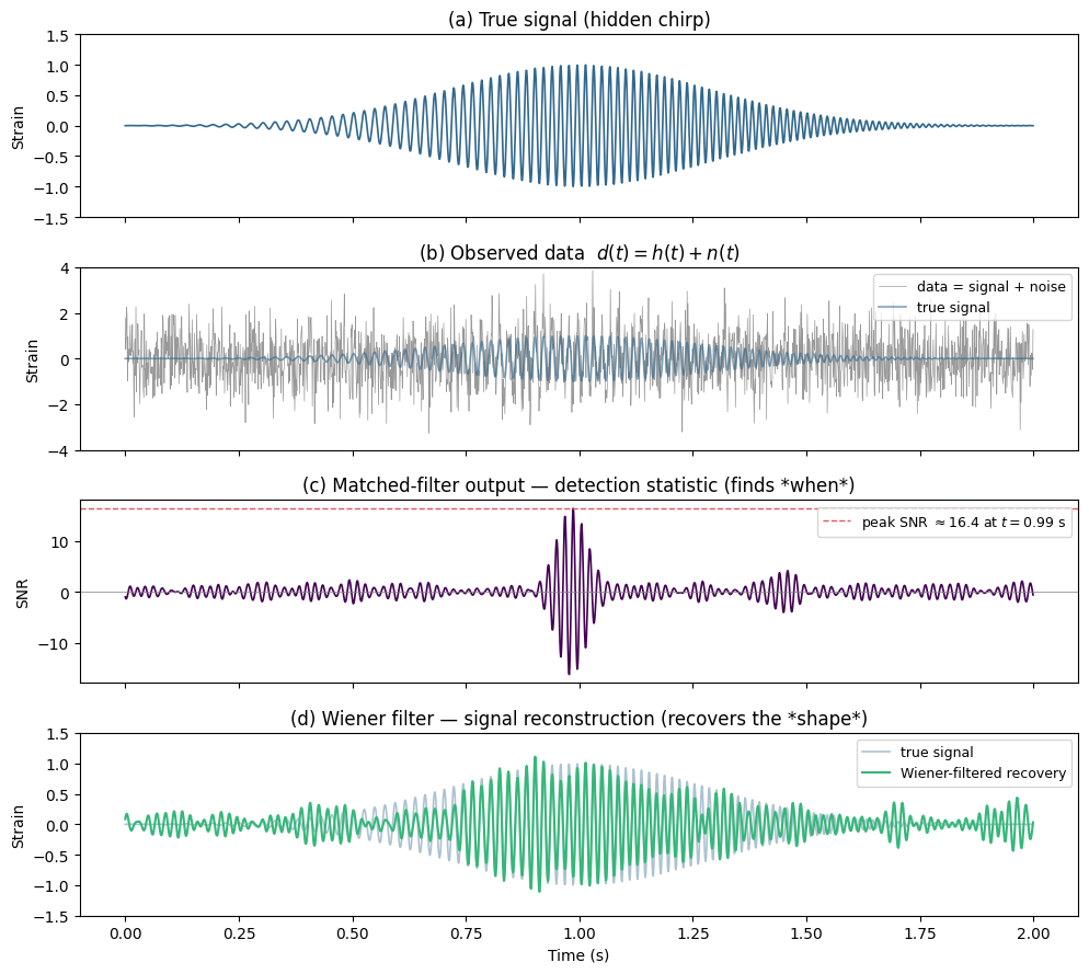
Panel (c): Matched filter peaks at SNR ≈ 16.4 — it finds the arrival time.
Panel (d): Wiener filter reconstructs the signal shape and duration from the noisy data.
GWFish computes the optimal SNR (panel c). Real PE pipelines also reconstruct waveforms (panel d).
1. Load the GRB Catalogue#
We load the GRB catalogue produced in Tutorial 2 (structured jet model, no artificial cuts). This catalogue contains the redshift and viewing angle of each detected GRB.
cat_path = Path("Output_files/tutorial2_structured/simulated_catalogue.csv")
grb_cat  = pd.read_csv(cat_path)

print(f"Loaded catalogue with {len(grb_cat)} events")
print(f"Columns: {list(grb_cat.columns)}")
grb_cat.head()
Loaded catalogue with 716 events
Columns: ['z', 'theta_v', 'Ep_obs', 'Fp', 'T90']
| z | theta_v | Ep_obs | Fp | T90 | |
|---|---|---|---|---|---|
| 0 | 1.415636 | 1.255996 | 1599.774032 | 3.326475 | 0.303101 |
| 1 | 4.289053 | 1.154894 | 256.338163 | 0.751587 | 0.982531 |
| 2 | 1.185732 | 0.726972 | 512.985027 | 1.304992 | 1.782053 |
| 3 | 1.006062 | 4.975575 | 355.805279 | 4.290123 | 0.135932 |
| 4 | 1.436368 | 1.906071 | 1173.864785 | 1.195041 | 1.919871 |
Background: Waveform Physics & Binary Parameters#
The SNR formula above depends on the signal \(\tilde{h}(f)\), which is completely determined by the source parameters. Here we review the key physics that connects the parameters in our catalogue to the shape of the GW signal.
Polarisations#
A compact binary coalescence (CBC) produces two independent polarisations of GW strain:
where \(\iota\) is the inclination angle (= \(\theta_{jn}\) from our GRB catalogue), \(d_L\) is the luminosity distance, \(\Phi(t)\) is the orbital phase, and \(\mathcal{M}_c\) is the chirp mass:
The chirp mass is the best-measured parameter in GW observations because it controls the leading-order frequency evolution of the signal \(\dot{f} \propto \mathcal{M}_c^{5/3} f^{11/3}\).
Redshift and the Mass–Distance Degeneracy#
GW detectors measure redshifted (“detector-frame”) masses, not the source-frame masses:
Since the luminosity distance \(d_L\) and redshift \(z\) are linked by cosmology, a further, heavier binary produces nearly the same waveform as a closer, lighter one. This mass–distance degeneracy is a fundamental limitation of GW-only observations and is one reason why electromagnetic counterparts (like the sGRBs from our catalogue) are so valuable — they independently constrain \(z\).
2. Generate BNS Parameters#
For each event in the catalogue we need the full set of parameters required by GWFish. We draw masses from a Gaussian distribution centred on the Galactic double-NS population (\(\mu = 1.33\,M_\odot\), \(\sigma = 0.09\,M_\odot\)) and randomise sky position, polarisation, phase, and GPS time. The viewing angle \(\theta_{jn}\) comes directly from the catalogue.
n_ev     = len(grb_cat)
redshift = grb_cat["z"].values

# Viewing angle from the GRB catalogue (stored in degrees → convert to radians for GWFish)
theta_jn = np.deg2rad(grb_cat["theta_v"].values)

# BNS masses — Gaussian (Galactic DNS population)
m1, m2 = np.random.normal(1.33, 0.09, (n_ev, 2)).T
# Enforce m1 >= m2
mass_1 = np.maximum(m1, m2)
mass_2 = np.minimum(m1, m2)

# Extrinsic parameters (randomised)
params_dict = {
    "mass_1_source"        : mass_1,
    "mass_2_source"        : mass_2,
    "redshift"             : redshift,
    "luminosity_distance"  : Planck18.luminosity_distance(redshift).value,
    "theta_jn"             : theta_jn,
    "ra"                   : np.random.uniform(0.0, 2 * np.pi, n_ev),
    "dec"                  : np.arcsin(np.random.uniform(-1.0, 1.0, n_ev)),
    "psi"                  : np.random.uniform(0.0, np.pi, n_ev),
    "phase"                : np.random.uniform(0.0, 2 * np.pi, n_ev),
    "geocent_time"         : np.random.uniform(1577491218, 1609027217, n_ev),
    "a_1"                  : np.zeros(n_ev),
    "a_2"                  : np.zeros(n_ev),
}

df_params = pd.DataFrame(params_dict)

# Save the generated parameters for reproducibility
df_params.to_csv(output_dir / "bns_params.csv", index=False)

print(f"Generated {n_ev} BNS parameter sets")
print(f"  <m1> = {mass_1.mean():.3f} Msun,  <m2> = {mass_2.mean():.3f} Msun")
print(f"  z ∈ [{redshift.min():.3f}, {redshift.max():.3f}]")
df_params.head()
Generated 716 BNS parameter sets
  <m1> = 1.383 Msun,  <m2> = 1.276 Msun
  z ∈ [0.077, 7.138]
| mass_1_source | mass_2_source | redshift | luminosity_distance | theta_jn | ra | dec | psi | phase | geocent_time | a_1 | a_2 | |
|---|---|---|---|---|---|---|---|---|---|---|---|---|
| 0 | 1.346837 | 1.263713 | 1.415636 | 10423.384411 | 0.021921 | 2.226126 | -0.477595 | 2.562928 | 3.816972 | 1.601854e+09 | 0.0 | 0.0 |
| 1 | 1.528181 | 1.215226 | 4.289053 | 39810.647221 | 0.020157 | 5.970543 | 0.464268 | 0.070029 | 4.852231 | 1.598927e+09 | 0.0 | 0.0 |
| 2 | 1.327049 | 1.229784 | 1.185732 | 8378.321342 | 0.012688 | 3.643638 | 0.582195 | 0.495682 | 4.362396 | 1.605754e+09 | 0.0 | 0.0 |
| 3 | 1.465627 | 1.238579 | 1.006062 | 6842.022386 | 0.086840 | 4.521687 | 0.377468 | 1.641903 | 0.963937 | 1.607602e+09 | 0.0 | 0.0 |
| 4 | 1.288927 | 1.256483 | 1.436368 | 10611.625959 | 0.033267 | 4.527660 | -0.586511 | 0.936680 | 1.943180 | 1.596175e+09 | 0.0 | 0.0 |
Background: The Fisher Information Matrix (the “Fish” in GWFish)#
GWFish doesn’t just compute SNR — it can also estimate how well each parameter can be measured. Here we briefly sketch the underlying method. (Tutorial 4 will explore parameter estimation in more detail.)
From Bayes’ Theorem to the Likelihood#
Given data \(d\), the posterior on the source parameters \(\boldsymbol{\theta}\) is:
where \(\mathcal{L}\) is the likelihood and \(\pi\) is the prior. For a Gaussian-noise detector, the log-likelihood is:
using the same noise-weighted inner product defined above.
The Gaussian Approximation (High-SNR Limit)#
In the high-SNR regime, the likelihood can be Taylor-expanded around the true parameters \(\hat{\boldsymbol{\theta}}\) and approximated as a multivariate Gaussian:
where \(\Delta \theta^i = \theta^i - \hat{\theta}^i\) and \(F_{ij}\) is the Fisher Information Matrix.
Fisher Matrix Elements#
The Fisher matrix is computed from the derivatives of the waveform with respect to each parameter:
Intuitively, if changing a parameter significantly alters the waveform (large \(\partial h / \partial \theta\)), then the data constrains that parameter tightly.
From Fisher to Parameter Errors#
The inverse of the Fisher matrix gives the covariance matrix:
and the off-diagonal terms encode correlations between parameters: \(\rho_{ij} = C_{ij} / (\sigma_i \sigma_j)\).
Note: In this tutorial we only use GWFish for SNR computation. In Tutorial 4, we will use the full Fisher matrix to estimate sky localisation and parameter uncertainties, and visualise parameter correlations with corner plots.
3. Set Up the GWFish Detector Network#
Background: Detector Response & Antenna Patterns#
A single detector does not measure \(h_+\) and \(h_\times\) independently. The measured strain is a linear combination weighted by the antenna pattern functions:
where \(F_+\) and \(F_\times\) depend on the source sky position (RA \(\alpha\), Dec \(\delta\)), polarisation angle \(\psi\), and the detector’s orientation and geometry. Every detector has blind spots — sky directions where \(F_+ \approx F_\times \approx 0\).
Network SNR#
For a network of \(N\) detectors, the total SNR is the quadrature sum of the individual detector SNRs:
Similarly, the Fisher information matrices add: \(F_{ij}^{\mathrm{net}} = \sum_k F_{ij}^{(k)}\), meaning more detectors always improve parameter estimation.
Why 3G Detectors (ET / CE)?#
Einstein Telescope (ET): Originally designed as a triangular underground detector, effectively equivalent to 3 co-located interferometers. The 2L configuration used here (two separated L-shaped detectors, ETS and ETN) reduces blind spots compared to a single L-shaped detector and provides independent noise realisations, improving both detection confidence and sky localisation.
Cosmic Explorer (CE): A 40 km L-shaped surface detector with extraordinary low-frequency sensitivity. When combined with ET, the long baseline (\(\sim\)5000 km) dramatically improves sky localisation via triangulation.
We start with the Einstein Telescope 2L configuration:
Detector |
Description |
|---|---|
|
Einstein Telescope — South, 15 km arms |
|
Einstein Telescope — North, 15 km arms |
import re, tempfile

# ---------- Detector configuration ----------
# Source YAML (contains bare PSD filenames like "ET_15_coba.txt")
yaml_template = Path("configs/coba.yaml")

# Directory containing the local PSD files
psd_dir = Path("psds").resolve()

def resolve_psd_paths(yaml_path, psd_dir):
    """Read a GWFish config YAML and resolve every bare `psd_data` filename
    to an absolute path under *psd_dir*. Returns the path to a temporary
    YAML file with all paths resolved. Makes it safe to pass to GWFish."""
    text = yaml_path.read_text()
    # Match `psd_data:` followed by a value that is NOT already an absolute path
    def _resolve(m):
        fname = m.group(1).strip()
        if fname.startswith("/"):        # already absolute → keep as-is
            return m.group(0)
        resolved = (psd_dir / fname).resolve()
        if not resolved.exists():
            raise FileNotFoundError(
                f"PSD file not found: {resolved}  (referenced in {yaml_path})"
            )
        return f"psd_data:{m.group(0).split('psd_data:')[1].replace(fname, str(resolved))}"
    resolved_text = re.sub(r"psd_data:\s*(.+)", _resolve, text)
    # Write to a temp file that GWFish can read
    tmp = tempfile.NamedTemporaryFile(
        mode="w", suffix=".yaml", prefix="gwfish_conf_", delete=False
    )
    tmp.write(resolved_text)
    tmp.flush()
    return Path(tmp.name)

conf_file = resolve_psd_paths(yaml_template, psd_dir)
print(f"Resolved config written to: {conf_file}")

# Network: ET 2L (South + North, 15 km arms)
detector_names = ["ETS_15", "ETN_15"]

waveform_model = "IMRPhenomD_NRTidalv2"

network = gw.detection.Network(
    detector_ids  = detector_names,
    config        = conf_file,
    detection_SNR = (0, 8),
)

# Quick sanity check: plot the PSDs
for det in network.detectors:
    det.components[0].plot_psd()
plt.legend(detector_names)
plt.title("PSD — ET 2L (ETS_15 + ETN_15)")
plt.savefig(output_dir / "PSDs.pdf")
plt.show()
print(f"Network initialised with detectors: {detector_names}")
Resolved config written to: /tmp/gwfish_conf_0epzmgi6.yaml
Network initialised with detectors: ['ETS_15', 'ETN_15']
4. Compute Network SNR (Multiprocessing)#
We compute the SNR for every event using gw.utilities.get_snr, split across all available CPU cores.
The last column of the returned array is the network (quadrature-summed) SNR.
from joblib import Parallel, delayed

my_pop_split = np.array_split(df_params, cpus)

def run_snr(chunk_df):
    return gw.utilities.get_snr(chunk_df, network=network, waveform_model=waveform_model)

snr_chunks = Parallel(n_jobs=cpus, verbose=10)(
    delayed(run_snr)(chunk) for chunk in my_pop_split
)

snr_array = np.concatenate(snr_chunks)   # shape: (n_ev, n_detectors + 1)

# Individual detector SNRs and network SNR
individual_snrs = snr_array[:, :-1]
network_snr     = snr_array[:, -1]

print(f"SNR computed for {len(network_snr)} events")
print(f"  Median network SNR : {np.median(network_snr):.1f}")
print(f"  Max    network SNR : {np.max(network_snr):.1f}")
[Parallel(n_jobs=12)]: Using backend LokyBackend with 12 concurrent workers.
[Parallel(n_jobs=12)]: Done   1 tasks      | elapsed:    5.5s
[Parallel(n_jobs=12)]: Done   3 out of  12 | elapsed:    5.7s remaining:   17.1s
[Parallel(n_jobs=12)]: Done   5 out of  12 | elapsed:    5.7s remaining:    8.0s
[Parallel(n_jobs=12)]: Done   7 out of  12 | elapsed:    5.8s remaining:    4.1s
[Parallel(n_jobs=12)]: Done   9 out of  12 | elapsed:    5.9s remaining:    2.0s
SNR computed for 716 events
  Median network SNR : 10.1
  Max    network SNR : 144.7
[Parallel(n_jobs=12)]: Done 12 out of 12 | elapsed: 6.1s finished
Fallback: Single-Process SNR Computation#
If multiprocessing causes issues (e.g., on some systems or inside containers), uncomment and run the cell below instead of the multiprocessing cell above.
# # --- Single-process fallback (uncomment if multiprocessing fails) ---
# snr_array   = gw.utilities.get_snr(df_params, network=network, waveform_model=waveform_model)
#
# individual_snrs = np.array(snr_array)[:, :-1]
# network_snr     = np.array(snr_array)[:, -1]
#
# print(f"SNR computed for {len(network_snr)} events (single process)")
# print(f"  Median network SNR : {np.median(network_snr):.1f}")
# print(f"  Max    network SNR : {np.max(network_snr):.1f}")
5. Detection Rate & Redshift Distribution#
Background: Detection Threshold & Statistics#
Why SNR > 8?#
In real GW data, noise fluctuations can occasionally mimic a signal. For Gaussian noise, the amplitude of these fluctuations follows a \(\chi^2\) distribution. The threshold \(\rho > 8\) is chosen so that the probability of a pure noise fluctuation exceeding this value — the false alarm rate (FAR) — is negligibly small (roughly one false trigger per \(\sim 10^5\) years for a single template). This ensures that any event crossing the threshold is almost certainly astrophysical.
Detection Efficiency#
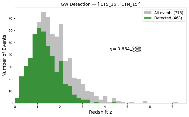
The detection fraction (or efficiency) is:
Since detection is a counting process, the uncertainty on \(N_{\mathrm{det}}\) follows Poisson statistics: \(\Delta N_{\mathrm{det}} = \sqrt{N_{\mathrm{det}}}\), giving:
By comparing the redshift distribution of all events vs. detected events, we can directly see how \(\eta(z)\) decreases with distance — the SNR scales as \(\rho \propto 1/d_L\), so distant mergers progressively fall below threshold.
SNR_THRESHOLD = 8.0

detected_mask   = network_snr > SNR_THRESHOLD
total_events    = len(network_snr)
detected_events = int(np.sum(detected_mask))

# Poisson uncertainty on the detection count
poisson_err = np.sqrt(detected_events)
ratio       = detected_events / total_events
ratio_plus  = (detected_events + poisson_err) / total_events
ratio_minus = (detected_events - poisson_err) / total_events

print(f"{detector_names} detected {detected_events} / {total_events}  (SNR > {SNR_THRESHOLD})")
print(f"Detection rate: {ratio:.3f}  [{ratio_minus:.3f}, {ratio_plus:.3f}]")

# ---- Redshift histogram ----
bins = np.linspace(0, redshift.max() + 0.5, 40)

fig, ax = plt.subplots(figsize=(8, 5))
ax.hist(redshift, bins=bins, color="gray", alpha=0.5,
        label=f"All events ({total_events})")
ax.hist(redshift[detected_mask], bins=bins, color="green", alpha=0.7,
        label=f"Detected ({detected_events})")
ax.text(
    0.55, 0.55,
    f"$\\eta = {{{ratio:.3f}}}^{{+{ratio_plus - ratio:.3f}}}_{{-{ratio - ratio_minus:.3f}}}$",
    transform=ax.transAxes, fontsize=13,
)
ax.set_xlabel("Redshift $z$", fontsize=14)
ax.set_ylabel("Number of Events", fontsize=14)
ax.set_title(f"GW Detection — {detector_names}", fontsize=13)
ax.set_xlim(0, redshift.max() + 0.5)
ax.legend(fontsize=11)
plt.tight_layout()
plt.savefig(output_dir / "detection_redshift_hist.pdf", dpi=300, bbox_inches="tight")
plt.show()
['ETS_15', 'ETN_15'] detected 468 / 716  (SNR > 8.0)
Detection rate: 0.654  [0.623, 0.684]
6. Save Results#
Save the full catalogue augmented with the network SNR and the detection mask so it can be used downstream (e.g., for joint GW+GRB population studies).
# Augment the original catalogue with SNR info
results_df = grb_cat.copy()
for i, det_name in enumerate(detector_names):
    results_df[f"snr_{det_name}"] = individual_snrs[:, i]
results_df["snr_network"] = network_snr
results_df["detected"]    = detected_mask

# Save
results_df.to_csv(output_dir / "catalogue_with_snr.csv", index=False)

print(f"Saved augmented catalogue to {output_dir / 'catalogue_with_snr.csv'}")
print(f"Columns: {list(results_df.columns)}")
results_df.head()
Saved augmented catalogue to Output_files/tutorial3_gwfish/catalogue_with_snr.csv
Columns: ['z', 'theta_v', 'Ep_obs', 'Fp', 'T90', 'snr_ETS_15', 'snr_ETN_15', 'snr_network', 'detected']
| z | theta_v | Ep_obs | Fp | T90 | snr_ETS_15 | snr_ETN_15 | snr_network | detected | |
|---|---|---|---|---|---|---|---|---|---|
| 0 | 1.415636 | 1.255996 | 1599.774032 | 3.326475 | 0.303101 | 7.726760 | 7.209373 | 10.567775 | True |
| 1 | 4.289053 | 1.154894 | 256.338163 | 0.751587 | 0.982531 | 4.781149 | 4.897866 | 6.844595 | False |
| 2 | 1.185732 | 0.726972 | 512.985027 | 1.304992 | 1.782053 | 4.422111 | 7.932813 | 9.082102 | True |
| 3 | 1.006062 | 4.975575 | 355.805279 | 4.290123 | 0.135932 | 15.546504 | 14.500249 | 21.259140 | True |
| 4 | 1.436368 | 1.906071 | 1173.864785 | 1.195041 | 1.919871 | 11.219100 | 10.699508 | 15.503150 | True |
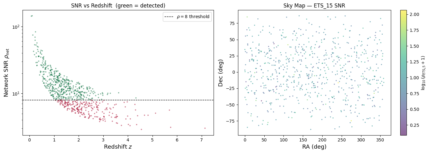
Diagnostic Plots#
Let’s visualise the results to build physical intuition. The left panel shows redshift vs. network SNR — you should see the expected \(\rho \propto 1/d_L \sim 1/z\) scaling. The right panel shows a sky map coloured by individual detector SNR, revealing the antenna pattern’s directional sensitivity.
fig, axes = plt.subplots(1, 2, figsize=(14, 5))

# --- Left: Redshift vs Network SNR (the 1/d_L scaling) ---
ax = axes[0]
sc = ax.scatter(redshift, network_snr, c=detected_mask, cmap="RdYlGn",
                s=8, alpha=0.5, edgecolors="none")
ax.axhline(SNR_THRESHOLD, ls="--", color="k", lw=1, label=rf"$\rho = {SNR_THRESHOLD:.0f}$ threshold")
ax.set_yscale("log")
ax.set_xlabel("Redshift $z$", fontsize=13)
ax.set_ylabel("Network SNR $\\rho_{\\mathrm{net}}$", fontsize=13)
ax.set_title("SNR vs Redshift  (green = detected)", fontsize=12)
ax.legend(fontsize=10)

# --- Right: Sky map coloured by SNR of the first detector ---
ax = axes[1]
ra_plot  = np.rad2deg(df_params["ra"].values)
dec_plot = np.rad2deg(df_params["dec"].values)
sc2 = ax.scatter(ra_plot, dec_plot, c=np.log10(individual_snrs[:, 0] + 1),
                 cmap="viridis", s=6, alpha=0.6, edgecolors="none")
cbar = plt.colorbar(sc2, ax=ax, label=rf"$\log_{{10}}(\rho_{{{detector_names[0]}}} + 1)$")
ax.set_xlabel("RA (deg)", fontsize=13)
ax.set_ylabel("Dec (deg)", fontsize=13)
ax.set_title(f"Sky Map — {detector_names[0]} SNR", fontsize=12)

plt.tight_layout()
plt.savefig(output_dir / "diagnostic_snr_sky.pdf", dpi=200, bbox_inches="tight")
plt.show()
Exercise: Add Cosmic Explorer to the Network#
Now it’s your turn! Re-run the detection analysis with an expanded network that includes
CE40 (Cosmic Explorer, 40 km arms) alongside the two ET detectors.
Steps:
Inspect the available detectors in the configuration file (printed below).
Define a new
detector_nameslist that includesCE40.Build a new
Network, compute SNRs, and compare the detection rate to the ET-only result.
Hint: You only need to change detector_names and re-run the SNR computation.
# Print all available detector entries from the configuration YAML
print("Available detectors in coba.yaml:")
print("=" * 40)
with open(yaml_template) as f:
    for line in f:
        # Print top-level detector names (no leading whitespace, ending with ':')
        stripped = line.rstrip()
        if stripped and not stripped.startswith(" ") and not stripped.startswith("#") and stripped.endswith(":"):
            print(f"  • {stripped[:-1]}")
Available detectors in coba.yaml:
========================================
  • ET
  • ETS_15
  • ETN_15
  • CE40
  • CE20
# ============================================================
# EXERCISE: Define the extended network and compute SNRs
# ============================================================

# TODO: Add CE40 to the detector list
detector_names_ext = ["ETS_15", "ETN_15"]  # <-- modify this line!

network_ext = gw.detection.Network(
    detector_ids  = detector_names_ext,
    config        = conf_file,
    detection_SNR = (0, 8),
)

# Compute SNR (single-process for simplicity; swap for joblib version if you prefer)
snr_array_ext   = gw.utilities.get_snr(df_params, network=network_ext, waveform_model=waveform_model)
network_snr_ext = np.array(snr_array_ext)[:, -1]

detected_ext = int(np.sum(network_snr_ext > SNR_THRESHOLD))
ratio_ext    = detected_ext / total_events

print(f"Extended network: {detector_names_ext}")
print(f"  Detected {detected_ext} / {total_events}  (SNR > {SNR_THRESHOLD})")
print(f"  Detection rate: {ratio_ext:.3f}")
print(f"\nOriginal ET-only rate: {ratio:.3f}")
print(f"Improvement factor:   {ratio_ext / ratio:.2f}x" if ratio > 0 else "")
Extended network: ['ETS_15', 'ETN_15']
  Detected 468 / 716  (SNR > 8.0)
  Detection rate: 0.654

Original ET-only rate: 0.654
Improvement factor:   1.00x
Summary#
In this notebook we:
Reviewed the theory of matched filtering, the noise-weighted inner product, and the optimal SNR
Connected source parameters to the GW signal: chirp mass, inclination, redshifted masses, and tidal deformability
Introduced the Fisher matrix as GWFish’s approximation to the likelihood (explored further in Tutorial 4)
Explained detector networks: antenna patterns, network SNR as a quadrature sum, and why ET + CE improves coverage
Built a pipeline: loaded GRB catalogues, generated BNS parameters, computed SNR with GWFish
Applied a detection threshold (\(\rho > 8\)) with Poisson uncertainties and visualised the redshift-dependent detection efficiency
Exercise: Extended the network with CE40 and compared detection rates.