Cosmo Tutorial

This is a brief guide on how to use GWFish to produce cosmological inferences

#! pip install -q git+https://github.com/janosch314/GWFish.git
#! pip install -q lalsuite
#! pip install -q corner
#! pip install -q dill
#! pip install -q getdist

Import packages

# suppress warning outputs for using lal in jupuyter notebook
import warnings 
warnings.filterwarnings("ignore", "Wswiglal-redir-stdio")

import GWFish.modules as gw
from tqdm import tqdm
import matplotlib
import matplotlib.pyplot as plt
import corner
import numpy as np
import pandas as pd
import json
import os
import dill as pickle
from getdist import loadMCSamples
import getdist.plots as gdplt
from scipy.integrate import simpson
import astropy.cosmology as apcosmo
from scipy.interpolate import interp1d

# plotting settings
matplotlib.rcParams.update({
    'font.size': 10,
    'axes.labelsize': 10,
    'axes.titlesize': 16,
    'xtick.labelsize': 10,
    'ytick.labelsize': 10,
    'legend.fontsize': 10,
    'figure.titlesize': 14
})

Let’s create suitable catalog of events

from_deg_to_rad = np.pi/180.

def create_dir(path):
    if not os.path.exists(path):
        os.makedirs(path)
        print('Directory created: ', path)
    else:
        pass
        #print('Directory already exists: ', path)

ns = 80
np.random.seed(42)

unphysical approach

# data = {}
# data['redshift'] = np.random.uniform(0.001, 3, ns)
# mass_1_source = np.random.uniform(low = 1.1, high = 2.1, size = ns)
# mass_2_source = np.random.uniform(low = 1.1, high = 2.1, size = ns)
# data['luminosity_distance'] = np.ones(len(data['redshift']))#dL_z(data['redshift'])
# data['ra'] = np.random.uniform(0., 2 * np.pi, ns)
# data['dec'] = np.arcsin(np.random.uniform(-1., 1., ns))
# data['psi'] = np.random.uniform(0., np.pi, ns)
# data['phase'] = np.random.uniform(0., 2 * np.pi, ns)
# data['geocent_time'] = np.random.uniform(1577491218, 1609027217, ns)

physical approach

def md_merger_rate(z, alphaF, betaF, CF, norm):
    return norm * (1+z)**alphaF / (1+((1+z)/CF)**betaF) 

def sampling_redshift_bns(redshift_dict, NSamples, seed):

    #choosing the cosmology
    keys = list(redshift_dict.keys())
    if 'Om0' in keys:  
        Om0 = redshift_dict['Om0']
    else:              
        Om0 = None
    if 'Ode0' in keys: 
        Ode0 = redshift_dict['Ode0']
    else:              
        Ode0 = None
    if 'H0' in keys:   
        H0 = redshift_dict['H0']
    else:              
        H0 = None

    if None in (Om0,Ode0,H0):
        cosmo = apcosmo.Planck18
    else:
        cosmo = apcosmo.LambdaCDM(H0=H0, Om0=Om0, Ode0=Ode0)

    # Initializing the random number generator    
    rng = np.random.default_rng(seed)

    # uniform redshift distribution
    if redshift_dict['model'] == 'uniform':
        if redshift_dict['default'] == True:
            zmin = 0.
            zmax = 10.
        else:
            zmin = redshift_dict['zmin']
            zmax = redshift_dict['zmax']

        z_vec = rng.uniform(low=zmin, high=zmax, size=NSamples)

    # uniform in comoving volume
    elif redshift_dict['model'] == 'uniform_comoving_volume':
        if redshift_dict['default'] == True:
            zmin = 0.
            zmax = 10.
        else:
            zmin = redshift_dict['zmin']
            zmax = redshift_dict['zmax']

        nzs = max(5001, 50 * int((zmax-zmin)) + 1)
        zs = np.linspace(zmin,zmax,nzs)
        z_dist = (lambda z: ((4.*np.pi*cosmo.differential_comoving_volume(z).value)/(1.+z)))(zs)
        window_cdf = np.array([simpson(z_dist[:i],zs[:i]) for i in range(1,nzs+1)]) / simpson(z_dist,zs)
        inv_window_cdf = interp1d(window_cdf, zs)
        z_vec = inv_window_cdf(rng.random(NSamples))

    # Madau-Dickinson merger rate, with fiducial parameters come from the GWBENCH package
    elif redshift_dict['model'] == 'madau_dickinson':
        if redshift_dict['default'] == True:
            zmin   = 0.
            zmax   = 10.
            alphaF = 1.803219571
            betaF  = 5.309821767
            CF     = 2.837264101
            norm   = 8.765949529
        else:
            zmin   = redshift_dict['zmin']
            zmax   = redshift_dict['zmax']
            alphaF = redshift_dict['alphaF']
            betaF  = redshift_dict['betaF']
            CF     = redshift_dict['CF']
            norm   = redshift_dict['norm']

        nzs = max(5001, 50 * int((zmax-zmin)) + 1)
        zs = np.linspace(zmin,zmax,nzs)
        z_dist = (lambda z: ((md_merger_rate(z,alphaF,betaF,CF,norm)*4.*np.pi*cosmo.differential_comoving_volume(z).value)/(1.+z)))(zs)
        window_cdf = np.array([simpson(z_dist[:i],zs[:i]) for i in range(1,nzs+1)]) / simpson(z_dist,zs)
        inv_window_cdf = interp1d(window_cdf, zs)
        z_vec = inv_window_cdf(rng.random(NSamples))

    DL_vec = cosmo.luminosity_distance(z_vec).value

    return z_vec, DL_vec

redshift_dict = {
    'model' : 'madau_dickinson',
    'default' : True
}

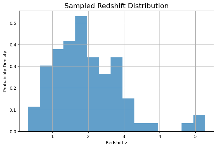
z_samples, dL_samples = sampling_redshift_bns(redshift_dict, ns, seed=42)

#plot z_samples
plt.figure(figsize=(8,5))
plt.hist(z_samples, bins=15, density=True, alpha=0.7)
plt.xlabel('Redshift z')
plt.ylabel('Probability Density')
plt.title('Sampled Redshift Distribution')
plt.grid()
plt.show()

# sort the two masses so that m1>m2 and create M_chirp and q

mass_1_source = np.random.uniform(low = 1.1, high = 2.1, size = ns)
mass_2_source = np.random.uniform(low = 1.1, high = 2.1, size = ns)

mass_1_det = mass_1_source * (1+z_samples)
mass_2_det = mass_2_source * (1+z_samples)

aux_mass = mass_1_det
mass_1_det = np.maximum(aux_mass, mass_2_det)
mass_2_det = np.minimum(aux_mass, mass_2_det)

#create only visible GRBs

a, b, c, d = -1., np.cos(175/180*np.pi), np.cos(5/180*np.pi), 1.

# Specify relative probabilities
prob = np.array([b-a, d-c])
prob = prob/prob.sum() # Normalize to sum up to one

r = []
for ii in range(ns):
    r.append(np.random.choice([np.arccos(np.random.uniform(a, b)), np.arccos(np.random.uniform(c, d))], p=prob))

theta_data = np.array(r)

data = {}
data['redshift'] = z_samples
data['mass_ratio'] = mass_2_det/mass_1_det
data['chirp_mass'] = (mass_1_det * mass_2_det)**(3/5) / (mass_1_det + mass_2_det)**(1/5)
data['luminosity_distance'] = dL_samples
data['ra'] = np.random.uniform(0., 2 * np.pi, ns)
data['dec'] = np.arcsin(np.random.uniform(-1., 1., ns))
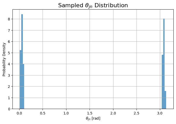
data['theta_jn'] = theta_data
data['psi'] = np.random.uniform(0., np.pi, ns)
data['phase'] = np.random.uniform(0., 2 * np.pi, ns)
data['geocent_time'] = np.random.uniform(1577491218, 1609027217, ns)

# plot theta_jn
plt.figure(figsize=(8,5))
plt.hist(data['theta_jn'], bins=100, density=True, alpha=0.7)
plt.xlabel(r'$\theta_{jn}$ [rad]')
plt.ylabel('Probability Density')
plt.title(r'Sampled $\theta_{jn}$ Distribution')
plt.grid()
plt.show()

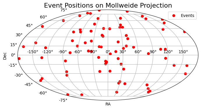
plt.figure(figsize=(8, 5)) 
ra_rad = data['ra'].astype(float) 

# Shift RA from [0, 2pi] to [-pi, pi] for mollweide 
ra_rad = np.where(ra_rad > np.pi, ra_rad - 2 * np.pi, ra_rad) 

dec_rad = data['dec'].astype(float) 

ax = plt.subplot(111, projection='mollweide') 
ax.scatter(ra_rad, dec_rad, marker='o', color='red', label='Events') 

ax.grid(True) 
ax.set_xlabel('RA') 
ax.set_ylabel('Dec') 
ax.set_title('Event Positions on Mollweide Projection') 
plt.legend() 
plt.show()

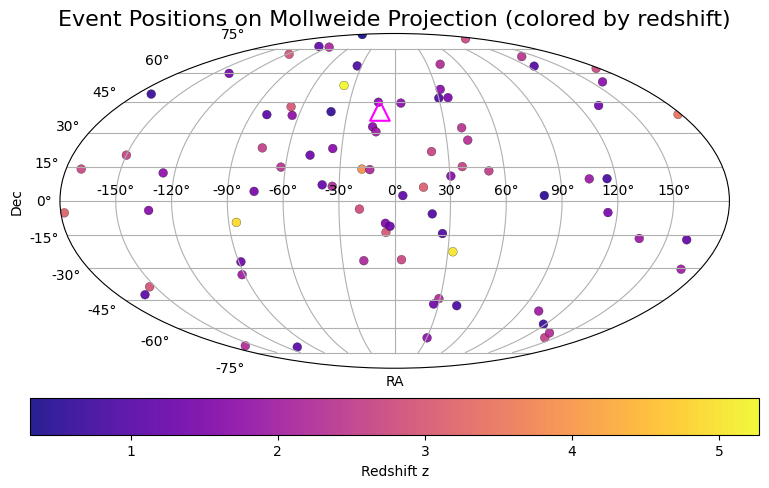
lat_ET = (40 + 31./60) * np.pi / 180.   # radians
lon_ET = (9 + 25./60) * np.pi / 180.    # radians

x_ET = -lon_ET   # flip longitude to match RA convention
y_ET = lat_ET

plt.figure(figsize=(8, 5)) 
ra_rad = data['ra'].astype(float) 

# Shift RA from [0, 2pi] to [-pi, pi] for mollweide 
ra_rad = np.where(ra_rad > np.pi, ra_rad - 2 * np.pi, ra_rad) 

dec_rad = data['dec'].astype(float) 
z_vals = data['redshift'].astype(float)

ax = plt.subplot(111, projection='mollweide') 

# scatter with colormap based on redshift
sc = ax.scatter(ra_rad, dec_rad, c=z_vals, cmap='plasma', s=40, edgecolors='k', linewidths=0.2, alpha=0.9)
ax.scatter(x_ET, y_ET, marker='^', s=200, facecolors='none', edgecolors='magenta', linewidths=1.5, label='ET delta')

ax.grid(True) 
ax.set_xlabel('RA') 
ax.set_ylabel('Dec') 
ax.set_title('Event Positions on Mollweide Projection (colored by redshift)') 

# colorbar
cb = plt.colorbar(sc, ax=ax, orientation='horizontal', pad=0.07)
cb.set_label('Redshift z')

plt.tight_layout()
plt.show()

data2save = pd.DataFrame(data=data)
data2save.head(5)

	redshift	mass_ratio	chirp_mass	luminosity_distance	ra	dec	theta_jn	psi	phase	geocent_time
0	2.649630	0.751127	5.394567	22404.316540	0.647946	0.261777	0.052906	2.211932	0.126111	1.607083e+09
1	1.641375	0.840340	4.319453	12502.973009	5.670907	0.402258	0.083231	0.669047	2.023683	1.583207e+09
2	3.149753	0.781060	5.840114	27580.417558	3.174594	-0.091044	3.092178	0.428424	1.328567	1.579588e+09
3	2.341390	0.684987	4.074958	19290.559269	5.192785	0.257968	3.074520	0.045693	2.057727	1.600863e+09
4	0.802911	0.890173	2.088720	5185.199461	2.010931	0.169438	0.076745	1.101403	0.752488	1.595608e+09

catalog_folder = os.path.join(os.getcwd(), "output")

create_dir(catalog_folder)

data2save.to_hdf(catalog_folder + f'/grb_events.hdf5', mode='w', key='root')

Let’s use GWFish! We will first use raw GWFish and then apply physical priors

np.random.seed(42)

population = 'BNS'
networks = '[[0]]' 
detectors = ['ET']
networks_ids = json.loads(networks)

ConfigDet = ' '

threshold_SNR =  (0., 8.)

waveform_model = 'IMRPhenomHM'

fisher_parameters = ['chirp_mass', 'mass_ratio', 'luminosity_distance', 'theta_jn', 'psi', 'phase'] 

corner_lbs = ['$\mathcal{M}_c$ $[M_{\odot}]$', '$q$', '$d_L$ [Mpc]', '$\iota$ [rad]', '$\Psi$ [rad]', '$\phi$ [rad]']

parameters = pd.read_hdf(catalog_folder + f'/grb_events.hdf5')
parameters.head(5)

	redshift	mass_ratio	chirp_mass	luminosity_distance	ra	dec	theta_jn	psi	phase	geocent_time
0	2.649630	0.751127	5.394567	22404.316540	0.647946	0.261777	0.052906	2.211932	0.126111	1.607083e+09
1	1.641375	0.840340	4.319453	12502.973009	5.670907	0.402258	0.083231	0.669047	2.023683	1.583207e+09
2	3.149753	0.781060	5.840114	27580.417558	3.174594	-0.091044	3.092178	0.428424	1.328567	1.579588e+09
3	2.341390	0.684987	4.074958	19290.559269	5.192785	0.257968	3.074520	0.045693	2.057727	1.600863e+09
4	0.802911	0.890173	2.088720	5185.199461	2.010931	0.169438	0.076745	1.101403	0.752488	1.595608e+09

kwargs_network = {'detector_ids': detectors}


path_out_GWFish = os.path.join(os.getcwd(), "output", "gwfish_results")

if threshold_SNR is not None:
    kwargs_network['detection_SNR'] = threshold_SNR
if ConfigDet!= ' ':
    kwargs_network['config'] = ConfigDet

network = gw.detection.Network(**kwargs_network)

gw.fishermatrix.analyze_and_save_to_txt(network = network,
                                        parameter_values  = parameters,
                                        fisher_parameters = fisher_parameters, 
                                        sub_network_ids_list = networks_ids,
                                        population_name = population,
                                        waveform_model = waveform_model,
                                        save_path = path_out_GWFish,
                                        save_matrices = True,
                                        use_duty_cycle = True)

100%|██████████| 80/80 [00:14<00:00,  5.53it/s]

Let’s apply physical priors

# join detector entries with underscore
detectors_str = '_'.join(detectors)
det = detectors_str  # alias used later in the notebook

file_path = path_out_GWFish + f'/Errors_{detectors_str}_{population}_SNR{int(threshold_SNR[1])}.txt'


# Read header line (strip leading '#' or '//' and commas) and load data
with open(file_path, 'r') as f:
    header = f.readline().lstrip('#/ \t').replace(',', ' ')
cols = header.split()

means = pd.read_csv(file_path, names=cols, skiprows=1, delim_whitespace=True)

cov_path = os.path.join(path_out_GWFish, f'inv_fisher_matrices_{detectors_str}_{population}_SNR{int(threshold_SNR[1])}.npy')
cov_matrix = np.load(cov_path)

lbs_mns = fisher_parameters

z_thr = 0.13
check_z_thr = means[means['redshift'] < z_thr]

CornerPlot = False
plotPosteriors = False
DensityPlot = False
PlotPeculiar = False

# if check_z_thr is empty then skip

if check_z_thr.empty:
    include_vp = False
else:
    include_vp = True

Example of Applications

See Figure 1 in Cozzumbo, et al. 2024

mns = means[lbs_mns]
NN = len(mns)
N = 100_000
zmax = max(means['redshift'])

m1min = 1.1
m2min = 1.1
m1max = 2.5 * (1+zmax)
m2max = 2.5 * (1+zmax)

event_list = []
z_list  = []
density_list = []
skipped_events = []
posterior_list = []
dl_inject = []
Ddl_inject = []

save_density = None

min_array = np.array([0.,     0.01, 0.,      0.,    0.,    0.      ])
max_array = np.array([100.,   1.,   np.inf,  np.pi, np.pi, 2*np.pi ])

#from GWFish.modules.priors import *

from priors_mine import *
from scipy.stats import norm

mother_dir = os.getcwd()

# for each event we proceed to the truncation and then to the prior evaluation and posterior sampling from a physically motivated prior-informed likelihood

for event in tqdm(np.arange(NN)):

    mns_ev = mns.iloc[event].to_numpy()
    cov_ev = cov_matrix[event, :, :]
    rng = np.random.default_rng(seed=100)

    fisher_samples = pd.DataFrame(rng.multivariate_normal(mns_ev, cov_ev, N), columns = fisher_parameters)
    
    # TRUNCATED SAMPLING

    try:
        with warnings.catch_warnings():
            warnings.simplefilter("error")  # Convert warnings into exceptions
            
            samples_truncated_mvn = get_truncated_likelihood_samples(
                fisher_parameters, mns_ev, cov_ev, N, 
                min_array=min_array, max_array=max_array
            )

    except Warning as w:  # Catch warnings
        print(f"Warning in truncated evaluation: {w}")
        skipped_events.append([means['redshift'][int(event)]])
        continue  # Skip to the next iteration

    except Exception as e:  # Catch other exceptions
        print(f"Error in truncated evaluation: {e}")
        skipped_events.append([means['redshift'][int(event)]])
        continue


    priors_dict = get_default_priors_dict(fisher_parameters) 

    # Chirp mass prior


    # Luminosity distance prior
    priors_dict['luminosity_distance']['prior_type'] = "uniform_in_comoving_volume_and_source_frame"
    
    priors_dict['luminosity_distance']['lower_prior_bound'] = 10


    priors_dict['luminosity_distance']['upper_prior_bound'] = 50000


    priors_dict['chirp_mass']['prior_type'] ='uniform_in_component_masses_chirp_mass'

    priors_dict['chirp_mass']['lower_prior_bound'] = ((m1min * m2min)**(3/5) / (m1min + m2min)**(1/5)) 

    priors_dict['chirp_mass']['upper_prior_bound'] = ((m1max * m2max)**(3/5) / (m1max + m2max)**(1/5))

    # theta_jn prior
    priors_dict['theta_jn']['prior_type'] = "uniform_in_sine"
    theta_jn_lowerbound = 0.
    theta_jn_upperbound = 5.

    if 0 < means['theta_jn'][event] < np.pi/2 :
        priors_dict['theta_jn']['lower_prior_bound'] = theta_jn_lowerbound*np.pi/180.
                    
    else:
        priors_dict['theta_jn']['lower_prior_bound'] = (180-theta_jn_upperbound)*np.pi/180


    if 0 < means['theta_jn'][event] < np.pi/2 :
        priors_dict['theta_jn']['upper_prior_bound'] = theta_jn_upperbound*np.pi/180.
                    
    else:
        priors_dict['theta_jn']['upper_prior_bound'] = (180-theta_jn_lowerbound)*np.pi/180


    # PRIOR EVALUATION and POSTERIOR SAMPLING

    try:
        samples_from_posterior = get_posteriors_samples(fisher_parameters, samples_truncated_mvn, N, priors_dict = priors_dict)
        
    except Exception as e:
        print('Error in the prior evaluation:', e)
        skipped_events.append([means['redshift'][int(event)]])
        continue

    z_save = means['redshift'][int(event)]

                    
    if CornerPlot:

        CORNER_KWARGS = dict(
                            bins = 50, # number of bins for histograms
                            smooth = 0.99, # smooths out contours. 
                            plot_datapoints = False, # choose if you want datapoints
                            truth_color='red',
                            label_kwargs = dict(fontsize = 16), # font size for labels
                            show_titles = True, #choose if you want titles on top of densities.
                            title_kwargs = dict(fontsize = 12), # font size for title
                            plot_density = True,
                            title_quantiles = [0.16, 0.5, 0.84],  # add quantiles to plot densities for 1d hist
                            levels = (1 - np.exp(-0.5), 1 - np.exp(-2), 1 - np.exp(-9 / 2.)), # 1, 2 and 3 sigma contours for 2d plots
                            fill_contours = True, #decide if you want to fill the contours
                            max_n_ticks = 3, # set a limit to ticks in the x-y axes.
                            title_fmt=".2f"
                            )
        
        fig = corner.corner(fisher_samples, labels = corner_lbs, truths = mns_ev, color = 'black', alpha = 0.5, **CORNER_KWARGS)
        old_fig = corner.corner(samples_truncated_mvn, labels = corner_lbs, truths = mns_ev, color = 'orange', alpha = 0.5, **CORNER_KWARGS, fig = fig)
        new_fig = corner.corner(samples_from_posterior, labels = corner_lbs, truths = mns_ev, color = 'red', alpha = 0.5, **CORNER_KWARGS, fig = fig)
        

        plot_dir = f"{mother_dir}/check_images/corner"
        create_dir(plot_dir)
        plt.savefig(plot_dir + f'/cornerplot_{event}.pdf',dpi=600, bbox_inches='tight', facecolor='white')

        plt.close()

    if plotPosteriors:

        # Set font size for ticks
        matplotlib.rc('xtick', labelsize=8)
        matplotlib.rc('ytick', labelsize=8)

        # Create subplots
        fig, axs = plt.subplots(2, 3, figsize=(10, 10))

        # Histogram plots
        params = fisher_parameters
        positions = [(0, 0), (0, 1), (0, 2), (1, 0), (1, 1), (1, 2)]

        for param, pos in zip(params, positions):
            counts, edges, _ = axs[pos].hist(samples_from_posterior[param].to_numpy(), bins=50)
            axs[pos].set_xlabel(param, fontsize=8)
            
            # Plot injected values
            axs[pos].axvline(x=mns_ev[params.index(param)], color='red', label='injected')
            
            # Plot new mean values
            axs[pos].axvline(x=samples_from_posterior[param].mean(), color='orange', label='new mean')
            
            # Plot max posterior values
            mode_index = np.argmax(counts)
            axs[pos].axvline(x=0.5 * (edges[mode_index] + edges[mode_index + 1]), color='lightgreen', label='max posterior')

        # Adjust layout and add legend
        plt.legend(bbox_to_anchor=(1., 0.5), loc='center left', fontsize=8)
        plt.tight_layout()

        # Save plot
        target_dir = f"{mother_dir}/check_images/posteriors"
        create_dir(target_dir)
        plt.savefig(f'{target_dir}/GW_posteriors_{event}.pdf', dpi=600, bbox_inches='tight', facecolor='white')

        # Close figure
        plt.close()


    # here we save the posterior samples for the luminosity distance only, to be used in the cosmological analysis
    # we use getdist kde interpolation, that is fast and flexible
    # SAVE ALL POSTERIORS
    
    weights, edges, _ = plt.hist(samples_from_posterior['luminosity_distance'].to_numpy(), bins=100, density=True)
    plt.close()

    out_path_posteriors = f"{mother_dir}/output/posteriors"
    create_dir(out_path_posteriors)
    final_samples = np.zeros((3,len(samples_from_posterior['luminosity_distance'].to_numpy())))
    final_samples[0, :] = 1
    final_samples[2,:] = samples_from_posterior['luminosity_distance'].to_numpy()
    # CREATE PARAMFILE
    param_list = ['d_L']
    paramfile = [param_list[ii] + '\t' + param_list[ii] for ii in range(len(param_list))]
    np.savetxt(out_path_posteriors + f'/posteriors_tmp.paramnames', paramfile, fmt='%s')
    
    np.savetxt(out_path_posteriors+ f'/posteriors_tmp.txt', np.transpose(final_samples), fmt='%i %.6e %.6e')
    settings = {'smooth_scale_1D' : 0.3}
    sample_getdist=gdplt.loadMCSamples(out_path_posteriors + f'/posteriors_tmp', settings=settings)
    density = gdplt.MCSamples.get1DDensityGridData(sample_getdist, 0)

    z_list.append(z_save)
    
    density_list.append(density)
    if DensityPlot:
        plt.rc('font', size=25, family='serif')
        plt.rc('text', usetex=True)
        fig = plt.figure(figsize=(10, 10))
        xx = np.linspace(min(samples_from_posterior['luminosity_distance'].to_numpy()), max(samples_from_posterior['luminosity_distance'].to_numpy()),300)
        plt.hist(samples_from_posterior['luminosity_distance'].to_numpy(), bins=100, density=True, alpha=0.7)
        plt.plot(xx, max(weights)*density(xx), lw=3, label= 'Interpolating density')
        #plt.plot(xx, max(weights)*density2(xx), label= 'Interpolating density bw=0.3')
        plt.legend()

        plot_dir =  f"{mother_dir}/check_images/density"
        create_dir(plot_dir)
        plt.tight_layout()
        plt.xlabel(r'$z$')
        plt.ylabel(r'$p(d_L)$')
        plt.savefig(plot_dir + f'/densityplot_{z_save}_{event}.pdf',dpi=600, bbox_inches='tight', facecolor='white')
        #plt.show()
        plt.close()

    # just to save the posteriors
    posterior_list.append(samples_from_posterior['luminosity_distance'].to_numpy())
    dl_inject.append(means['luminosity_distance'].to_numpy()[event])
    Ddl_inject.append(means['err_luminosity_distance'].to_numpy()[event])


    
out_path_kde = f"{mother_dir}/output/kde"
create_dir(out_path_kde)

# if there are elements with z < z_thr, then we apply the correction

if include_vp:
    print('Peculiar velocity correction on going')
    print('Starting the peculiar velocity analysis\n')
    # include vp correction
    
    dt = {}
    dt['z'] = z_list
    dt['posterior'] = posterior_list
    dt['kde'] = density_list
    dt['dl'] = dl_inject
    dt['Ddl'] = Ddl_inject
    dataframe_data = pd.DataFrame(data=dt)                
    sorted_df = dataframe_data.sort_values(by=['z'])
    idx_cycle = np.where(np.array(sorted_df['z']) <= z_thr)[0]


    mean_vp = 300.
    sigma_vp = 200.
    
    if len(idx_cycle) != 0:
        
        for idx, ii in enumerate(idx_cycle):
            
            gw_samples = sorted_df['posterior'].to_numpy()[ii]
            gw_density = sorted_df['kde'].to_numpy()[ii]
            z_event = sorted_df['z'].to_numpy()[ii]
            dl= sorted_df['dl'].to_numpy()[ii]
            Ddl= sorted_df['Ddl'].to_numpy()[ii]
            rng = np.random.RandomState(ii)
            vp_rms = rng.normal(loc=mean_vp, scale=50) 
            sigma_vp = rng.normal(loc=sigma_vp, scale=50)
            
            sigma_dL_vp = np.median(gw_samples) * sigma_vp / (vp_rms + c * z_event) 
            #first estimate of the peculiar velocity distribution impedence when combined by 
            #simple quadrature sum because we need dL_values to be big enough
            peculiar_Ddl = np.sqrt((Ddl)**2 + sigma_dL_vp**2)
            if dl-3*peculiar_Ddl <=0:
                min_bound = 0
            else:
                min_bound = dl-3*peculiar_Ddl
            dL_values = np.linspace(min_bound, dl+3*peculiar_Ddl, 10000)
            # Generate a Gaussian distribution for the peculiar velocity part
            v_p_distribution = norm(loc=np.median(gw_samples), scale=sigma_dL_vp)
            # Calculate the PDF of the peculiar velocity part
            pdf_vp = v_p_distribution.pdf(dL_values)
            # Calculate the PDF of the combined distribution by convolving the PDFs
            combined_pdf = np.convolve(pdf_vp, gw_density(dL_values), mode='same')
            # Normalize the combined PDF
            combined_pdf /= np.sum(combined_pdf)
            histogram, bin_edges = np.histogram(dL_values, bins=10000, weights=combined_pdf)
            combined_samples = np.random.choice((bin_edges[:-1] + bin_edges[1:]) / 2, size=1_000_000, p= np.abs(histogram) / np.sum(histogram))
            samp = np.zeros((3,len(combined_samples)))
            samp[0, :] = 1
            samp[2,:] = combined_samples
            np.savetxt(out_path_posteriors+ f'/posteriors_tmp.txt', np.transpose(samp), fmt='%i %.6e %.6e')
            
            settings = {'smooth_scale_1D' :0.3}
            getdist=gdplt.loadMCSamples(out_path_posteriors+ f'/posteriors_tmp', settings=settings)
            density_final = gdplt.MCSamples.get1DDensityGridData(getdist, 0)
            
            dataframe_data['kde'] = density_final
            
            #Plot the combined distribution
            if PlotPeculiar:
                plt.figure(figsize=(10, 10))

                plt.plot(dL_values, density_final(dL_values), label=r'Combined kde with Gaussian $v_{\mathrm{peculiar}}$', color='green')
                plt.plot(dL_values, gw_density(dL_values), label='Old kde', color='red')
                plt.xlabel(r'$d_L$')
                plt.ylabel('Density')
                plt.title(f'Event at $z$={z_event} | $z_t$={z_thr} $v_p$={vp_rms:.2f} $\sigma_v$={sigma_vp:.2f}')
                plt.legend(loc='upper right')
                plt.xlim(np.min(gw_samples), np.max(gw_samples))

                plot_dir = f"{mother_dir}/check_images/peculiar_velocity"
                create_dir(plot_dir)
                plt.savefig(plot_dir + f'/peculiar_velocity_{idx}.pdf',dpi=600, bbox_inches='tight', facecolor='white')
                #plt.show()
                plt.close()
        
        density_vp = list(dataframe_data['kde'])
        
        save_density = [z_list, density_list, dl_inject, Ddl_inject, density_vp]

else:
    save_density = [z_list, density_list, dl_inject, Ddl_inject]
    
cosmology_save = 'LCDM_Planck18'
create_dir(out_path_kde + f'/{det}_{cosmology_save}_fiducial')

with open(out_path_kde + f'/{det}_{cosmology_save}_fiducial/{det}_{cosmology_save}_fiducial.pkl', 'wb') as handle:

    pickle.dump(save_density, handle, protocol=pickle.HIGHEST_PROTOCOL)

os.remove(out_path_posteriors + f'/posteriors_tmp.txt')


print(f'Max z seen: {max(z_list)}')
print('Skipped events [name, redshift]:', skipped_events)

  3%|▎         | 1/34 [09:37<5:17:32, 577.34s/it]

/Users/andreacozzumbo/GSSIprojects/acme_tutorials/cosmo_tutorial/output/posteriors/posteriors_tmp.txt
Removed no burn in

  6%|▌         | 2/34 [09:38<2:07:09, 238.43s/it]

/Users/andreacozzumbo/GSSIprojects/acme_tutorials/cosmo_tutorial/output/posteriors/posteriors_tmp.txt
Removed no burn in

  9%|▉         | 3/34 [09:39<1:39:50, 193.24s/it]

/Users/andreacozzumbo/GSSIprojects/acme_tutorials/cosmo_tutorial/output/posteriors/posteriors_tmp.txt
Removed no burn in

---------------------------------------------------------------------------
KeyboardInterrupt                         Traceback (most recent call last)
Cell In[31], line 75
     72 # PRIOR EVALUATION and POSTERIOR SAMPLING
     74 try:
---> 75     samples_from_posterior = get_posteriors_samples(fisher_parameters, samples_truncated_mvn, N, priors_dict = priors_dict)
     77 except Exception as e:
     78     print('Error in the prior evaluation:', e)

File ~/GSSIprojects/acme_tutorials/cosmo_tutorial/priors_mine.py:378, in get_posteriors_samples(params, likelihood_samples, num_posterior_samples, priors_dict, cosmology, dL_z)
    376 else:
    377     if priors_dict[var]['prior_type'] != 'uniform_in_differential_comoving_volume_Class':
--> 378         prior *= globals()[priors_dict[var]['prior_type']](likelihood_samples[var].to_numpy(), priors_dict[var]['lower_prior_bound'], priors_dict[var]['upper_prior_bound'])
    379     else:
    380         prior *= globals()[priors_dict[var]['prior_type']](cosmology, likelihood_samples[var].to_numpy(), priors_dict[var]['lower_prior_bound'], priors_dict[var]['upper_prior_bound'], dL_z)

File ~/GSSIprojects/acme_tutorials/cosmo_tutorial/priors_mine.py:134, in uniform_in_comoving_volume_and_source_frame(x, a, b)
    129 z = np.interp(x, dd, zz)
    131 # remember to divide const.c by 1000 to convert to km/s
    133 return np.where(np.logical_and(z >= aa, z <= bb), 
--> 134         cosmo.differential_comoving_volume(z).value * (x / (1 + z) + (const.c.value / 1000) * (1 + z) / (cosmo.H(0).value * cosmo.efunc(z)))**(-1) / (1 + z), 0)

File /opt/miniconda3/envs/acme_tutorials/lib/python3.10/site-packages/astropy/cosmology/flrw/base.py:1398, in FLRW.differential_comoving_volume(self, z)
   1378 def differential_comoving_volume(self, z):
   1379     """Differential comoving volume at redshift z.
   1380 
   1381     Useful for calculating the effective comoving volume.
   (...)
   1396         input redshift.
   1397     """
-> 1398     dm = self.comoving_transverse_distance(z)
   1399     return self._hubble_distance * (dm**2.0) / (self.efunc(z) << u.steradian)

File /opt/miniconda3/envs/acme_tutorials/lib/python3.10/site-packages/astropy/cosmology/flrw/base.py:1175, in FLRW.comoving_transverse_distance(self, z)
   1153 def comoving_transverse_distance(self, z):
   1154     r"""Comoving transverse distance in Mpc at a given redshift.
   1155 
   1156     This value is the transverse comoving distance at redshift ``z``
   (...)
   1173     This quantity is also called the 'proper motion distance' in some texts.
   1174     """
-> 1175     return self._comoving_transverse_distance_z1z2(0, z)

File /opt/miniconda3/envs/acme_tutorials/lib/python3.10/site-packages/astropy/cosmology/flrw/base.py:1200, in FLRW._comoving_transverse_distance_z1z2(self, z1, z2)
   1178 r"""Comoving transverse distance in Mpc between two redshifts.
   1179 
   1180 This value is the transverse comoving distance at redshift ``z2`` as
   (...)
   1197 This quantity is also called the 'proper motion distance' in some texts.
   1198 """
   1199 Ok0 = self._Ok0
-> 1200 dc = self._comoving_distance_z1z2(z1, z2)
   1201 if Ok0 == 0:
   1202     return dc

File /opt/miniconda3/envs/acme_tutorials/lib/python3.10/site-packages/astropy/cosmology/flrw/base.py:1110, in FLRW._comoving_distance_z1z2(self, z1, z2)
   1092 def _comoving_distance_z1z2(self, z1, z2):
   1093     """
   1094     Comoving line-of-sight distance in Mpc between objects at redshifts
   1095     ``z1`` and ``z2``.
   (...)
   1108         Comoving distance in Mpc between each input redshift.
   1109     """
-> 1110     return self._integral_comoving_distance_z1z2(z1, z2)

File /opt/miniconda3/envs/acme_tutorials/lib/python3.10/site-packages/astropy/cosmology/flrw/base.py:1151, in FLRW._integral_comoving_distance_z1z2(self, z1, z2)
   1134 def _integral_comoving_distance_z1z2(self, z1, z2):
   1135     """
   1136     Comoving line-of-sight distance in Mpc between objects at redshifts
   1137     ``z1`` and ``z2``. The comoving distance along the line-of-sight
   (...)
   1149         Comoving distance in Mpc between each input redshift.
   1150     """
-> 1151     return self._hubble_distance * self._integral_comoving_distance_z1z2_scalar(z1, z2)

File /opt/miniconda3/envs/acme_tutorials/lib/python3.10/site-packages/astropy/cosmology/utils.py:57, in vectorize_redshift_method.<locals>.wrapper(self, *args, **kwargs)
     55     return func(self, *zs, *args[nin:], **kwargs)
     56 # non-scalar. use vectorized func
---> 57 return wrapper.__vectorized__(self, *zs, *args[nin:], **kwargs)

File /opt/miniconda3/envs/acme_tutorials/lib/python3.10/site-packages/numpy/lib/function_base.py:2372, in vectorize.__call__(self, *args, **kwargs)
   2369     self._init_stage_2(*args, **kwargs)
   2370     return self
-> 2372 return self._call_as_normal(*args, **kwargs)

File /opt/miniconda3/envs/acme_tutorials/lib/python3.10/site-packages/numpy/lib/function_base.py:2365, in vectorize._call_as_normal(self, *args, **kwargs)
   2362     vargs = [args[_i] for _i in inds]
   2363     vargs.extend([kwargs[_n] for _n in names])
-> 2365 return self._vectorize_call(func=func, args=vargs)

File /opt/miniconda3/envs/acme_tutorials/lib/python3.10/site-packages/numpy/lib/function_base.py:2455, in vectorize._vectorize_call(self, func, args)
   2452 # Convert args to object arrays first
   2453 inputs = [asanyarray(a, dtype=object) for a in args]
-> 2455 outputs = ufunc(*inputs)
   2457 if ufunc.nout == 1:
   2458     res = asanyarray(outputs, dtype=otypes[0])

File /opt/miniconda3/envs/acme_tutorials/lib/python3.10/site-packages/astropy/cosmology/flrw/base.py:1132, in FLRW._integral_comoving_distance_z1z2_scalar(self, z1, z2)
   1112 @vectorize_redshift_method(nin=2)
   1113 def _integral_comoving_distance_z1z2_scalar(self, z1, z2, /):
   1114     """
   1115     Comoving line-of-sight distance between objects at redshifts ``z1`` and
   1116     ``z2``. Value in Mpc.
   (...)
   1130         Returns `float` if input scalar, `~numpy.ndarray` otherwise.
   1131     """
-> 1132     return quad(self._inv_efunc_scalar, z1, z2, args=self._inv_efunc_scalar_args)[0]

File /opt/miniconda3/envs/acme_tutorials/lib/python3.10/site-packages/scipy/integrate/_quadpack_py.py:459, in quad(func, a, b, args, full_output, epsabs, epsrel, limit, points, weight, wvar, wopts, maxp1, limlst, complex_func)
    456     return retval
    458 if weight is None:
--> 459     retval = _quad(func, a, b, args, full_output, epsabs, epsrel, limit,
    460                    points)
    461 else:
    462     if points is not None:

File /opt/miniconda3/envs/acme_tutorials/lib/python3.10/site-packages/scipy/integrate/_quadpack_py.py:606, in _quad(func, a, b, args, full_output, epsabs, epsrel, limit, points)
    604 if points is None:
    605     if infbounds == 0:
--> 606         return _quadpack._qagse(func,a,b,args,full_output,epsabs,epsrel,limit)
    607     else:
    608         return _quadpack._qagie(func, bound, infbounds, args, full_output, 
    609                                 epsabs, epsrel, limit)

KeyboardInterrupt: 

Let’s play with cosmology!

we generate a likelihood and we run a cosmological MCMC with cobaya

this is interfaced with a Einstein-Boltzmann solver called CLASS

#! pip install -q cobaya
#! pip install -q openmpi
#! pip install -q "mpi4py>=3"

import cobaya
from cobaya.run import run
from cobaya.yaml import yaml_load_file
import yaml

# installing CLASS
os.system(f"cobaya-install classy -p {mother_dir}/myclass")

[install] Installing external packages at '/Users/andreacozzumbo/GSSIprojects/acme_tutorials/cosmo_tutorial/myclass'
[install] The installation path has been written into the global config file: /Users/andreacozzumbo/Library/Application Support/cobaya/config.yaml

================================================================================
classy
================================================================================

[install] Checking if dependencies have already been installed...
[install] External dependencies for this component already installed.
[install] Doing nothing.

================================================================================
* Summary * 
================================================================================

[install] All requested components' dependencies correctly installed at /Users/andreacozzumbo/GSSIprojects/acme_tutorials/cosmo_tutorial/myclass

0

cosmology = 'LCDM_Planck18'

cosmo_data_path = os.path.join(mother_dir, "output", "kde", f"{det}_{cosmology}_fiducial")
pt_path = os.path.join(mother_dir, "cosmo_MCMC")
class_path = os.path.join(mother_dir, "myclass", "code", "classy")
output_path_MCMC = os.path.join(mother_dir, "cosmo_MCMC", "chains", "test1", "test")

input_yaml_path = os.path.join(mother_dir, "cosmo_MCMC", "input", "test.yaml")

#input_file = f"{mother_dir}/cosmo_MCMC/input/input.yaml"

base_config = {
    "theory": {
        "classy": {
            "path": class_path,
            "ignore_obsolete": True
        }
    },
    "likelihood": {
        "likelihood.MMcosmology": {
            "data_directory": cosmo_data_path,
            "python_path": pt_path,
            "gw_network": "ET",         
            "grb_dataset": "fiducial",    
            "fiducial_cosmology": "LCDM_Planck18",
            "interpolation_method": "kde",
        }
    },
    "params": {
        "omega_b": {
            "value": 0.0224,
            "latex": r"\Omega_\mathrm{b} h^2"
        },
        
        "Omega_cdm": {
            "prior": {"min": 0.05, "max": 0.7},
            "ref": {"dist": "norm", "loc": 0.26, "scale": 0.01},
            "proposal": 0.05,
            "latex": r"\Omega_\mathrm{c}"
        },
        "H0": {
            "prior": {"min": 20, "max": 100},
            "ref": {"dist": "norm", "loc": 67, "scale": 0.5},
            "proposal": 1.,
            "latex": "H_\mathrm{0}"
        },
        "Omega_m": {"latex": r"\Omega_\mathrm{m}"},
        "Omega_Lambda": {"latex": r"\Omega_\Lambda"}
    },
    "sampler": {
        "mcmc": {
            "max_tries": 10000000,
            #"covmat": '/home/cozzumbo/AC/Theseus/covmat/covmat_all.covmat',
            "Rminus1_stop": 0.01
        }
    },
    "output": output_path_MCMC
}

with open(input_yaml_path, "w") as f:
    yaml.dump(base_config, f, sort_keys=False)

input_file = input_yaml_path

os.system(f'mpirun -n 4 cobaya-run {input_file}')

[0 : output] Output to be read-from/written-into folder '/Users/andreacozzumbo/GSSIprojects/acme_tutorials/cosmo_tutorial/cosmo_MCMC/chains/test1', with prefix 'test'
[0 : classy] `classy` module loaded successfully from /Users/andreacozzumbo/GSSIprojects/acme_tutorials/cosmo_tutorial/myclass/code/classy/build/lib.macosx-11.0-arm64-cpython-310/classy
[2 : likelihood.mmcosmology] Initialized Einstein-Telescope Likelihood
[2 : likelihood.mmcosmology] Data file ET_LCDM_Planck18_fiducial.pkl read from /Users/andreacozzumbo/GSSIprojects/acme_tutorials/cosmo_tutorial/output/kde/ET_LCDM_Planck18_fiducial
Number of event:  34
[0 : likelihood.mmcosmology] Initialized Einstein-Telescope Likelihood
[0 : likelihood.mmcosmology] Data file ET_LCDM_Planck18_fiducial.pkl read from /Users/andreacozzumbo/GSSIprojects/acme_tutorials/cosmo_tutorial/output/kde/ET_LCDM_Planck18_fiducial
Number of event:  34
[1 : likelihood.mmcosmology] Initialized Einstein-Telescope Likelihood
[1 : likelihood.mmcosmology] Data file ET_LCDM_Planck18_fiducial.pkl read from /Users/andreacozzumbo/GSSIprojects/acme_tutorials/cosmo_tutorial/output/kde/ET_LCDM_Planck18_fiducial
Number of event:  34
[3 : likelihood.mmcosmology] Initialized Einstein-Telescope Likelihood
[3 : likelihood.mmcosmology] Data file ET_LCDM_Planck18_fiducial.pkl read from /Users/andreacozzumbo/GSSIprojects/acme_tutorials/cosmo_tutorial/output/kde/ET_LCDM_Planck18_fiducial
Number of event:  34
[3 : mcmc] Getting initial point... (this may take a few seconds)
[1 : mcmc] Getting initial point... (this may take a few seconds)
[0 : mcmc] Getting initial point... (this may take a few seconds)
[2 : mcmc] Getting initial point... (this may take a few seconds)
[1 : mcmc] Initial point: Omega_cdm:0.271878, H0:67.5321
[0 : mcmc] Initial point: Omega_cdm:0.277356, H0:67.06657
[2 : mcmc] Initial point: Omega_cdm:0.2724093, H0:66.86094
[3 : mcmc] Initial point: Omega_cdm:0.2689743, H0:66.95968
[0 : model] Measuring speeds... (this may take a few seconds)
[0 : model] Setting measured speeds (per sec): {likelihood.MMcosmology: 706.0, classy: 22.6}
[0 : mcmc] Covariance matrix not present. We will start learning the covariance of the proposal earlier: R-1 = 30 (would be 2 if all params loaded).
[0 : mcmc] Sampling!
[0 : mcmc] Progress @ 2025-10-30 16:22:45 : 1 steps taken, and 0 accepted.
[1 : mcmc] Progress @ 2025-10-30 16:22:45 : 1 steps taken, and 0 accepted.
[2 : mcmc] Progress @ 2025-10-30 16:22:45 : 1 steps taken, and 0 accepted.
[3 : mcmc] Progress @ 2025-10-30 16:22:45 : 1 steps taken, and 0 accepted.

/Users/andreacozzumbo/GSSIprojects/acme_tutorials/cosmo_tutorial/cosmo_MCMC/likelihood/MMcosmology.py:85: RuntimeWarning: invalid value encountered in log
  log_likelihood+=np.log(self.density[i](dL_th))
/Users/andreacozzumbo/GSSIprojects/acme_tutorials/cosmo_tutorial/cosmo_MCMC/likelihood/MMcosmology.py:85: RuntimeWarning: divide by zero encountered in log
  log_likelihood+=np.log(self.density[i](dL_th))
/Users/andreacozzumbo/GSSIprojects/acme_tutorials/cosmo_tutorial/cosmo_MCMC/likelihood/MMcosmology.py:85: RuntimeWarning: divide by zero encountered in log
  log_likelihood+=np.log(self.density[i](dL_th))
/Users/andreacozzumbo/GSSIprojects/acme_tutorials/cosmo_tutorial/cosmo_MCMC/likelihood/MMcosmology.py:85: RuntimeWarning: invalid value encountered in log
  log_likelihood+=np.log(self.density[i](dL_th))
/Users/andreacozzumbo/GSSIprojects/acme_tutorials/cosmo_tutorial/cosmo_MCMC/likelihood/MMcosmology.py:85: RuntimeWarning: invalid value encountered in log
  log_likelihood+=np.log(self.density[i](dL_th))
/Users/andreacozzumbo/GSSIprojects/acme_tutorials/cosmo_tutorial/cosmo_MCMC/likelihood/MMcosmology.py:85: RuntimeWarning: divide by zero encountered in log
  log_likelihood+=np.log(self.density[i](dL_th))
/Users/andreacozzumbo/GSSIprojects/acme_tutorials/cosmo_tutorial/cosmo_MCMC/likelihood/MMcosmology.py:85: RuntimeWarning: divide by zero encountered in log
  log_likelihood+=np.log(self.density[i](dL_th))
/Users/andreacozzumbo/GSSIprojects/acme_tutorials/cosmo_tutorial/cosmo_MCMC/likelihood/MMcosmology.py:85: RuntimeWarning: invalid value encountered in log
  log_likelihood+=np.log(self.density[i](dL_th))

[0 : mcmc] Learn + convergence test @ 80 samples accepted.
[0 : mcmc] Ready to check convergence and learn a new proposal covmat (waiting for the rest...)
[3 : mcmc] Learn + convergence test @ 80 samples accepted.
[3 : mcmc] Ready to check convergence and learn a new proposal covmat (waiting for the rest...)
[1 : mcmc] Learn + convergence test @ 80 samples accepted.
[1 : mcmc] Ready to check convergence and learn a new proposal covmat (waiting for the rest...)
[2 : mcmc] Learn + convergence test @ 80 samples accepted.
[2 : mcmc] Ready to check convergence and learn a new proposal covmat (waiting for the rest...)
[0 : mcmc] All chains are ready to check convergence and learn a new proposal covmat
[0 : mcmc]  - Acceptance rate: 0.210 = avg([0.2381, 0.2057, 0.1681, 0.2188])
[0 : mcmc]  - Convergence of means: R-1 = 0.275023 after 364 accepted steps = sum([100, 86, 80, 98])
[0 : mcmc]  - Updated covariance matrix of proposal pdf.

/Users/andreacozzumbo/GSSIprojects/acme_tutorials/cosmo_tutorial/cosmo_MCMC/likelihood/MMcosmology.py:85: RuntimeWarning: divide by zero encountered in log
  log_likelihood+=np.log(self.density[i](dL_th))
/Users/andreacozzumbo/GSSIprojects/acme_tutorials/cosmo_tutorial/cosmo_MCMC/likelihood/MMcosmology.py:85: RuntimeWarning: divide by zero encountered in log
  log_likelihood+=np.log(self.density[i](dL_th))
/Users/andreacozzumbo/GSSIprojects/acme_tutorials/cosmo_tutorial/cosmo_MCMC/likelihood/MMcosmology.py:85: RuntimeWarning: divide by zero encountered in log
  log_likelihood+=np.log(self.density[i](dL_th))
/Users/andreacozzumbo/GSSIprojects/acme_tutorials/cosmo_tutorial/cosmo_MCMC/likelihood/MMcosmology.py:85: RuntimeWarning: divide by zero encountered in log
  log_likelihood+=np.log(self.density[i](dL_th))

[0 : mcmc] Learn + convergence test @ 160 samples accepted.
[0 : mcmc] Ready to check convergence and learn a new proposal covmat (waiting for the rest...)
[2 : mcmc] Learn + convergence test @ 160 samples accepted.
[2 : mcmc] Ready to check convergence and learn a new proposal covmat (waiting for the rest...)
[1 : mcmc] Learn + convergence test @ 160 samples accepted.
[1 : mcmc] Ready to check convergence and learn a new proposal covmat (waiting for the rest...)
[3 : mcmc] Learn + convergence test @ 160 samples accepted.
[3 : mcmc] Ready to check convergence and learn a new proposal covmat (waiting for the rest...)
[0 : mcmc] All chains are ready to check convergence and learn a new proposal covmat
[0 : mcmc]  - Acceptance rate: 0.258 = avg([0.2966, 0.2441, 0.2795, 0.2015])
[0 : mcmc]  - Convergence of means: R-1 = 0.073604 after 684 accepted steps = sum([194, 165, 165, 160])
[0 : mcmc]  - Updated covariance matrix of proposal pdf.

/Users/andreacozzumbo/GSSIprojects/acme_tutorials/cosmo_tutorial/cosmo_MCMC/likelihood/MMcosmology.py:85: RuntimeWarning: divide by zero encountered in log
  log_likelihood+=np.log(self.density[i](dL_th))
/Users/andreacozzumbo/GSSIprojects/acme_tutorials/cosmo_tutorial/cosmo_MCMC/likelihood/MMcosmology.py:85: RuntimeWarning: divide by zero encountered in log
  log_likelihood+=np.log(self.density[i](dL_th))
/Users/andreacozzumbo/GSSIprojects/acme_tutorials/cosmo_tutorial/cosmo_MCMC/likelihood/MMcosmology.py:85: RuntimeWarning: divide by zero encountered in log
  log_likelihood+=np.log(self.density[i](dL_th))
/Users/andreacozzumbo/GSSIprojects/acme_tutorials/cosmo_tutorial/cosmo_MCMC/likelihood/MMcosmology.py:85: RuntimeWarning: divide by zero encountered in log
  log_likelihood+=np.log(self.density[i](dL_th))

[0 : mcmc] Learn + convergence test @ 240 samples accepted.
[0 : mcmc] Ready to check convergence and learn a new proposal covmat (waiting for the rest...)
[1 : mcmc] Learn + convergence test @ 240 samples accepted.
[1 : mcmc] Ready to check convergence and learn a new proposal covmat (waiting for the rest...)
[2 : mcmc] Learn + convergence test @ 240 samples accepted.
[2 : mcmc] Ready to check convergence and learn a new proposal covmat (waiting for the rest...)
[3 : mcmc] Learn + convergence test @ 240 samples accepted.
[3 : mcmc] Ready to check convergence and learn a new proposal covmat (waiting for the rest...)
[0 : mcmc] All chains are ready to check convergence and learn a new proposal covmat
[0 : mcmc]  - Acceptance rate: 0.303 = avg([0.3192, 0.3034, 0.3056, 0.2801])
[0 : mcmc]  - Convergence of means: R-1 = 0.041214 after 1003 accepted steps = sum([271, 249, 242, 241])
[0 : mcmc]  - Updated covariance matrix of proposal pdf.

/Users/andreacozzumbo/GSSIprojects/acme_tutorials/cosmo_tutorial/cosmo_MCMC/likelihood/MMcosmology.py:85: RuntimeWarning: divide by zero encountered in log
  log_likelihood+=np.log(self.density[i](dL_th))
/Users/andreacozzumbo/GSSIprojects/acme_tutorials/cosmo_tutorial/cosmo_MCMC/likelihood/MMcosmology.py:85: RuntimeWarning: divide by zero encountered in log
  log_likelihood+=np.log(self.density[i](dL_th))
/Users/andreacozzumbo/GSSIprojects/acme_tutorials/cosmo_tutorial/cosmo_MCMC/likelihood/MMcosmology.py:85: RuntimeWarning: divide by zero encountered in log
  log_likelihood+=np.log(self.density[i](dL_th))
/Users/andreacozzumbo/GSSIprojects/acme_tutorials/cosmo_tutorial/cosmo_MCMC/likelihood/MMcosmology.py:85: RuntimeWarning: divide by zero encountered in log
  log_likelihood+=np.log(self.density[i](dL_th))
/Users/andreacozzumbo/GSSIprojects/acme_tutorials/cosmo_tutorial/cosmo_MCMC/likelihood/MMcosmology.py:85: RuntimeWarning: invalid value encountered in log
  log_likelihood+=np.log(self.density[i](dL_th))
/Users/andreacozzumbo/GSSIprojects/acme_tutorials/cosmo_tutorial/cosmo_MCMC/likelihood/MMcosmology.py:85: RuntimeWarning: invalid value encountered in log
  log_likelihood+=np.log(self.density[i](dL_th))

[0 : mcmc] Learn + convergence test @ 320 samples accepted.
[0 : mcmc] Ready to check convergence and learn a new proposal covmat (waiting for the rest...)
[1 : mcmc] Learn + convergence test @ 320 samples accepted.
[1 : mcmc] Ready to check convergence and learn a new proposal covmat (waiting for the rest...)
[2 : mcmc] Learn + convergence test @ 320 samples accepted.
[2 : mcmc] Ready to check convergence and learn a new proposal covmat (waiting for the rest...)
[3 : mcmc] Learn + convergence test @ 320 samples accepted.
[3 : mcmc] Ready to check convergence and learn a new proposal covmat (waiting for the rest...)
[0 : mcmc] All chains are ready to check convergence and learn a new proposal covmat
[0 : mcmc]  - Acceptance rate: 0.316 = avg([0.3345, 0.3138, 0.3034, 0.3113])
[0 : mcmc]  - Convergence of means: R-1 = 0.010461 after 1343 accepted steps = sum([368, 331, 324, 320])
[0 : mcmc]  - Updated covariance matrix of proposal pdf.

/Users/andreacozzumbo/GSSIprojects/acme_tutorials/cosmo_tutorial/cosmo_MCMC/likelihood/MMcosmology.py:85: RuntimeWarning: divide by zero encountered in log
  log_likelihood+=np.log(self.density[i](dL_th))
/Users/andreacozzumbo/GSSIprojects/acme_tutorials/cosmo_tutorial/cosmo_MCMC/likelihood/MMcosmology.py:85: RuntimeWarning: divide by zero encountered in log
  log_likelihood+=np.log(self.density[i](dL_th))
/Users/andreacozzumbo/GSSIprojects/acme_tutorials/cosmo_tutorial/cosmo_MCMC/likelihood/MMcosmology.py:85: RuntimeWarning: divide by zero encountered in log
  log_likelihood+=np.log(self.density[i](dL_th))
/Users/andreacozzumbo/GSSIprojects/acme_tutorials/cosmo_tutorial/cosmo_MCMC/likelihood/MMcosmology.py:85: RuntimeWarning: divide by zero encountered in log
  log_likelihood+=np.log(self.density[i](dL_th))

[0 : mcmc] Learn + convergence test @ 400 samples accepted.
[0 : mcmc] Ready to check convergence and learn a new proposal covmat (waiting for the rest...)
[1 : mcmc] Learn + convergence test @ 400 samples accepted.
[1 : mcmc] Ready to check convergence and learn a new proposal covmat (waiting for the rest...)
[2 : mcmc] Learn + convergence test @ 400 samples accepted.
[2 : mcmc] Ready to check convergence and learn a new proposal covmat (waiting for the rest...)
[3 : mcmc] Learn + convergence test @ 400 samples accepted.
[3 : mcmc] Ready to check convergence and learn a new proposal covmat (waiting for the rest...)
[0 : mcmc] All chains are ready to check convergence and learn a new proposal covmat
[0 : mcmc]  - Acceptance rate: 0.312 = avg([0.3387, 0.3151, 0.2996, 0.2911])
[0 : mcmc]  - Convergence of means: R-1 = 0.016175 after 1690 accepted steps = sum([463, 425, 402, 400])
[0 : mcmc]  - Updated covariance matrix of proposal pdf.

/Users/andreacozzumbo/GSSIprojects/acme_tutorials/cosmo_tutorial/cosmo_MCMC/likelihood/MMcosmology.py:85: RuntimeWarning: divide by zero encountered in log
  log_likelihood+=np.log(self.density[i](dL_th))
/Users/andreacozzumbo/GSSIprojects/acme_tutorials/cosmo_tutorial/cosmo_MCMC/likelihood/MMcosmology.py:85: RuntimeWarning: divide by zero encountered in log
  log_likelihood+=np.log(self.density[i](dL_th))
/Users/andreacozzumbo/GSSIprojects/acme_tutorials/cosmo_tutorial/cosmo_MCMC/likelihood/MMcosmology.py:85: RuntimeWarning: divide by zero encountered in log
  log_likelihood+=np.log(self.density[i](dL_th))
/Users/andreacozzumbo/GSSIprojects/acme_tutorials/cosmo_tutorial/cosmo_MCMC/likelihood/MMcosmology.py:85: RuntimeWarning: divide by zero encountered in log
  log_likelihood+=np.log(self.density[i](dL_th))
/Users/andreacozzumbo/GSSIprojects/acme_tutorials/cosmo_tutorial/cosmo_MCMC/likelihood/MMcosmology.py:85: RuntimeWarning: invalid value encountered in log
  log_likelihood+=np.log(self.density[i](dL_th))

[1 : mcmc] Progress @ 2025-10-30 16:23:45 : 1657 steps taken, and 442 accepted.
[2 : mcmc] Progress @ 2025-10-30 16:23:45 : 1644 steps taken, and 418 accepted.
[0 : mcmc] Progress @ 2025-10-30 16:23:45 : 1652 steps taken, and 475 accepted.
[3 : mcmc] Progress @ 2025-10-30 16:23:45 : 1641 steps taken, and 417 accepted.

/Users/andreacozzumbo/GSSIprojects/acme_tutorials/cosmo_tutorial/cosmo_MCMC/likelihood/MMcosmology.py:85: RuntimeWarning: divide by zero encountered in log
  log_likelihood+=np.log(self.density[i](dL_th))
/Users/andreacozzumbo/GSSIprojects/acme_tutorials/cosmo_tutorial/cosmo_MCMC/likelihood/MMcosmology.py:85: RuntimeWarning: divide by zero encountered in log
  log_likelihood+=np.log(self.density[i](dL_th))
/Users/andreacozzumbo/GSSIprojects/acme_tutorials/cosmo_tutorial/cosmo_MCMC/likelihood/MMcosmology.py:85: RuntimeWarning: divide by zero encountered in log
  log_likelihood+=np.log(self.density[i](dL_th))

[0 : mcmc] Learn + convergence test @ 480 samples accepted.
[0 : mcmc] Ready to check convergence and learn a new proposal covmat (waiting for the rest...)

/Users/andreacozzumbo/GSSIprojects/acme_tutorials/cosmo_tutorial/cosmo_MCMC/likelihood/MMcosmology.py:85: RuntimeWarning: divide by zero encountered in log
  log_likelihood+=np.log(self.density[i](dL_th))
/Users/andreacozzumbo/GSSIprojects/acme_tutorials/cosmo_tutorial/cosmo_MCMC/likelihood/MMcosmology.py:85: RuntimeWarning: invalid value encountered in log
  log_likelihood+=np.log(self.density[i](dL_th))
/Users/andreacozzumbo/GSSIprojects/acme_tutorials/cosmo_tutorial/cosmo_MCMC/likelihood/MMcosmology.py:85: RuntimeWarning: invalid value encountered in log
  log_likelihood+=np.log(self.density[i](dL_th))

[1 : mcmc] Learn + convergence test @ 480 samples accepted.
[1 : mcmc] Ready to check convergence and learn a new proposal covmat (waiting for the rest...)
[3 : mcmc] Learn + convergence test @ 480 samples accepted.
[3 : mcmc] Ready to check convergence and learn a new proposal covmat (waiting for the rest...)
[2 : mcmc] Learn + convergence test @ 480 samples accepted.
[2 : mcmc] Ready to check convergence and learn a new proposal covmat (waiting for the rest...)
[0 : mcmc] All chains are ready to check convergence and learn a new proposal covmat
[0 : mcmc]  - Acceptance rate: 0.284 = avg([0.2993, 0.2887, 0.2679, 0.2760])
[0 : mcmc]  - Convergence of means: R-1 = 0.008902 after 2023 accepted steps = sum([539, 517, 480, 487])
[0 : mcmc]  - Updated covariance matrix of proposal pdf.

/Users/andreacozzumbo/GSSIprojects/acme_tutorials/cosmo_tutorial/cosmo_MCMC/likelihood/MMcosmology.py:85: RuntimeWarning: divide by zero encountered in log
  log_likelihood+=np.log(self.density[i](dL_th))
/Users/andreacozzumbo/GSSIprojects/acme_tutorials/cosmo_tutorial/cosmo_MCMC/likelihood/MMcosmology.py:85: RuntimeWarning: divide by zero encountered in log
  log_likelihood+=np.log(self.density[i](dL_th))
/Users/andreacozzumbo/GSSIprojects/acme_tutorials/cosmo_tutorial/cosmo_MCMC/likelihood/MMcosmology.py:85: RuntimeWarning: divide by zero encountered in log
  log_likelihood+=np.log(self.density[i](dL_th))
/Users/andreacozzumbo/GSSIprojects/acme_tutorials/cosmo_tutorial/cosmo_MCMC/likelihood/MMcosmology.py:85: RuntimeWarning: divide by zero encountered in log
  log_likelihood+=np.log(self.density[i](dL_th))

[0 : mcmc] Learn + convergence test @ 560 samples accepted.
[0 : mcmc] Ready to check convergence and learn a new proposal covmat (waiting for the rest...)

/Users/andreacozzumbo/GSSIprojects/acme_tutorials/cosmo_tutorial/cosmo_MCMC/likelihood/MMcosmology.py:85: RuntimeWarning: invalid value encountered in log
  log_likelihood+=np.log(self.density[i](dL_th))

[1 : mcmc] Learn + convergence test @ 560 samples accepted.
[1 : mcmc] Ready to check convergence and learn a new proposal covmat (waiting for the rest...)
[3 : mcmc] Learn + convergence test @ 560 samples accepted.
[3 : mcmc] Ready to check convergence and learn a new proposal covmat (waiting for the rest...)
[2 : mcmc] Learn + convergence test @ 560 samples accepted.
[2 : mcmc] Ready to check convergence and learn a new proposal covmat (waiting for the rest...)
[0 : mcmc] All chains are ready to check convergence and learn a new proposal covmat
[0 : mcmc]  - Acceptance rate: 0.269 = avg([0.2716, 0.2778, 0.2545, 0.2711])
[0 : mcmc]  - Convergence of means: R-1 = 0.003535 after 2351 accepted steps = sum([615, 604, 560, 572])
[0 : mcmc]  - Convergence of bounds: R-1 = 0.074825 after 2351 accepted steps = sum([615, 604, 560, 572])
[0 : mcmc] The run has converged!
[0 : mcmc] Sampling complete after 2351 accepted steps.

0

from getdist import loadMCSamples
from getdist import plots

import matplotlib as mpl
mpl.rcParams['text.usetex'] = False

settings = {'ignore_rows' : 0.3, 'smooth_scale_2D' : 0.5, 'smooth_scale_1D' : 0.5, 'contours':[0.68, 0.95, 0.997]}

samples = loadMCSamples(f"{mother_dir}/cosmo_MCMC/chains/test1/test", settings=settings)

WARNING:root:outlier fraction 0.02916160388821385 

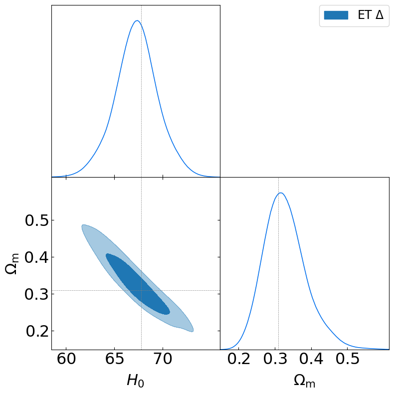
truth_LCDM={'Omega_m':0.309, 'Omega_cdm':0.26, 'H0':67.81}

g = plots.get_subplot_plotter()
g.settings.subplot_size_inch = 4
g.settings.legend_fontsize = 17
g.settings.axes_fontsize = 23

g.settings.lab_fontsize = 22

g.triangle_plot([samples],
                params=['H0', 'Omega_m'] ,
                filled=[True],
                markers=truth_LCDM,
                colors=['C0'],
                legend_labels = [r"ET $\Delta$"],
                legend_loc='upper right',
                )

from IPython.display import Math

def DisplayParamConstrain(chain, string_par=None, precision=3, string_before='', unit=''):
    stats = chain.getMargeStats()
    parstat = stats.parWithName(string_par)
    mean = parstat.mean
    lower = mean - parstat.limits[0].lower  # Limite inferiore
    upper = parstat.limits[0].upper - mean  # Limite superiore
    display(Math(rf"{string_before}{mean:.{precision}f}_{{-{lower:.{precision}f}}}^{{+{upper:.{precision}f}}}{unit}"))

DisplayParamConstrain(samples,'H0', string_before=r'H_\mathrm{0}: ', unit=r' \,\mathrm{km}\,\mathrm{s}^{-1}\,\mathrm{Mpc}^{-1}')  
DisplayParamConstrain(samples,'Omega_m', string_before=r'\Omega_\mathrm{m}:  ')

\[\displaystyle H_\mathrm{0}: 67.294_{-2.055}^{+2.079} \,\mathrm{km}\,\mathrm{s}^{-1}\,\mathrm{Mpc}^{-1}\]

\[\displaystyle \Omega_\mathrm{m}: 0.328_{-0.065}^{+0.047}\]