1. From basics to TDR

1. From basics to TDR#

This notebook builds the signal-analysis vocabulary needed for the Targeted Detectability Range (TDR), then traces the method and conclusions of Ronchini et al. (2026). The examples are synthetic and are not a search or an event analysis.

1.1 From a binary to a strain signal#

A compact binary inspiral loses orbital energy to gravitational radiation. Its orbital frequency rises, so the emitted GW “chirps” upward in frequency and amplitude before merger. A detector measures a dimensionless strain, approximately

\[d(t)=F_+(\alpha,\delta,\psi,t)h_+(t)+F_\times(\alpha,\delta,\psi,t)h_\times(t)+n(t),\]

where the antenna factors depend on sky position, polarization, and time, and \(n(t)\) is detector noise. Distance reduces the signal amplitude approximately as \(1/D_L\). Inclination changes the relative polarization amplitudes: a face-on binary is generally louder than an edge-on binary.

For a non-precessing, quasi-circular binary in the leading quadrupole approximation, a useful time-domain convention is

\[h_+(t)=A(t)\frac{1+\cos^2\iota}{2}\cos\Phi(t),\qquad h_\times(t)=A(t)\cos\iota\sin\Phi(t),\]

At Newtonian (leading quadrupole) order, the common amplitude scale can be written approximately as

\[A(t)=\frac{4}{D_L}\left(\frac{G\mathcal{M}}{c^2}\right)^{5/3}\left(\frac{\pi f_{\rm GW}(t)}{c}\right)^{2/3},\]

where \(D_L\) is luminosity distance, \(\mathcal{M}\) is chirp mass, and \(f_{\rm GW}\) is the instantaneous GW frequency. Neutron-star tides affect late inspiral; eccentricity and higher waveform modes can change the simple quadrupole shape and inclination dependence. These effects are why production analyses use full waveform models rather than just this scaling. \(\Phi(t)\) is the orbital/GW phase (up to convention), and \(\iota\) is the angle between the orbital angular-momentum axis and the line of sight.

At face-on (\(\iota=0\)), both angular factors are one: the signal is strongest and circularly polarized. At edge-on (\(\iota=90^\circ\)), the cross polarization vanishes and the plus factor is \(1/2\).

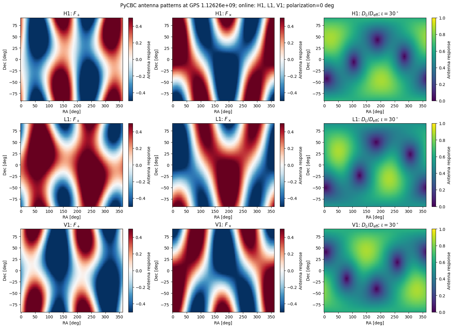
The measured strain is a second projection. \(F_+\) and \(F_\times\) are dimensionless antenna-pattern factors of a detector. They depend on the source direction (right ascension \(\alpha\), declination \(\delta\)), the wave polarization angle \(\psi\), the detector’s orientation, and the Earth’s rotation at observation time. Changing \(\psi\) rotates the plus/cross basis by twice that angle, mixing \(F_+\) and \(F_\times\); it does not change the source’s intrinsic radiation. The coalescence phase changes where the oscillation begins, while masses and spins set the chirp’s phase evolution and intrinsic amplitude. Thus sky position and time change how a detector views a waveform, not the binary’s emitted \(h_+\) and \(h_\times\).

Effective distance#

It is convenient to combine luminosity distance, antenna response, and inclination into the effective distance for one interferometer:

\[D_{\rm eff}=\frac{D_L}{\sqrt{F_+^2\left(\frac{1+\cos^2\iota}{2}\right)^2+F_\times^2\cos^2\iota}}. \]

The denominator is the source’s relative amplitude response (in the quadrupole, orthogonal-polarization approximation). A face-on overhead source can have \(D_{\rm eff}\simeq D_L\); an unfavorable sky location or edge-on orientation gives \(D_{\rm eff}>D_L\), and at an antenna null it diverges. For a fixed waveform and PSD, SNR scales approximately as \(1/D_{\rm eff}\). Effective distance is a useful way to compare projected amplitudes; it is not the source’s actual luminosity distance and by itself does not calculate the SNR.

The next cell displays the antenna pattern for the user-selected GPS time and online interferometers. Edit gps_time and online_ifos, then rerun the cell. It shows \(F_+\), \(F_\times\) and the inclination-dependent amplitude response over sky direction. The map uses PyCBC’s Detector.antenna_pattern function. This optional cell requires PyCBC (pip install pycbc); the core notebooks do not otherwise depend on it.

import numpy as np
import matplotlib.pyplot as plt

rng = np.random.default_rng(20261008)
def chirp_mass(m1, m2):
    """Return chirp mass in the same units as m1 and m2."""
    return (m1 * m2) ** (3 / 5) / (m1 + m2) ** (1 / 5)

chirp_mass(1.4, 1.4)

1.2187707886145736

# User choices: GPS time and interferometers online at that event time.
from pycbc.detector import Detector

gps_time = 1126259462.4  # GPS seconds
online_ifos = ["H1", "L1", "V1"]  # Edit this list as needed.
inclination_deg = 30.0
polarization_deg = 0.0

if not online_ifos:
    raise ValueError("Select at least one online interferometer")
if not np.isfinite(gps_time) or gps_time < 0:
    raise ValueError("gps_time must be finite and non-negative")
if not 0 <= inclination_deg <= 90:
    raise ValueError("inclination_deg must be between 0 and 90 degrees")

# PyCBC expects RA, declination, and polarization in radians, and time in GPS seconds.
ra, dec = np.meshgrid(np.deg2rad(np.linspace(0, 360, 121)),
                      np.deg2rad(np.linspace(-90, 90, 61)))
psi = np.deg2rad(polarization_deg)
iota = np.deg2rad(inclination_deg)
cos_iota = np.cos(iota)
a_plus = (1 + cos_iota**2) / 2
fig, axes = plt.subplots(len(online_ifos), 3, figsize=(15, 3.6 * len(online_ifos)),
                         squeeze=False, constrained_layout=True)

for row, ifo in enumerate(online_ifos):
    detector = Detector(ifo)
    # PyCBC evaluates one sky position per call; vectorize it over the sky grid.
    antenna_pattern = np.vectorize(
        lambda ra_rad, dec_rad: detector.antenna_pattern(ra_rad, dec_rad, psi, gps_time),
        otypes=[float, float],
    )
    f_plus, f_cross = antenna_pattern(ra, dec)
    response = np.sqrt((f_plus * a_plus)**2 + (f_cross * cos_iota)**2)
    fields = [
        (f_plus, r"$F_+$", "RdBu_r", -0.5, 0.5),
        (f_cross, r"$F_\times$", "RdBu_r", -0.5, 0.5),
        (response, rf"$D_L/D_{{\rm eff}}$; $\iota={inclination_deg:g}^\circ$", "viridis", 0, 1),
    ]
    for col, (values, title, cmap, vmin, vmax) in enumerate(fields):
        image = axes[row, col].pcolormesh(np.rad2deg(ra), np.rad2deg(dec), values,
                                          shading="auto", cmap=cmap, vmin=vmin, vmax=vmax)
        axes[row, col].set(xlabel="RA [deg]", ylabel="Dec [deg]", title=f"{ifo}: {title}")
        fig.colorbar(image, ax=axes[row, col], label="Antenna response")

fig.suptitle(f"PyCBC antenna patterns at GPS {gps_time:g}; online: {', '.join(online_ifos)}; "
             f"polarization={polarization_deg:g} deg")
plt.show()

../_images/fae6457832588fa089e7ea2e846f6d7ae12bd68d5a8138de8d70d1e3ccf484b0.png

1.2 Noise, PSD, and matched filtering#

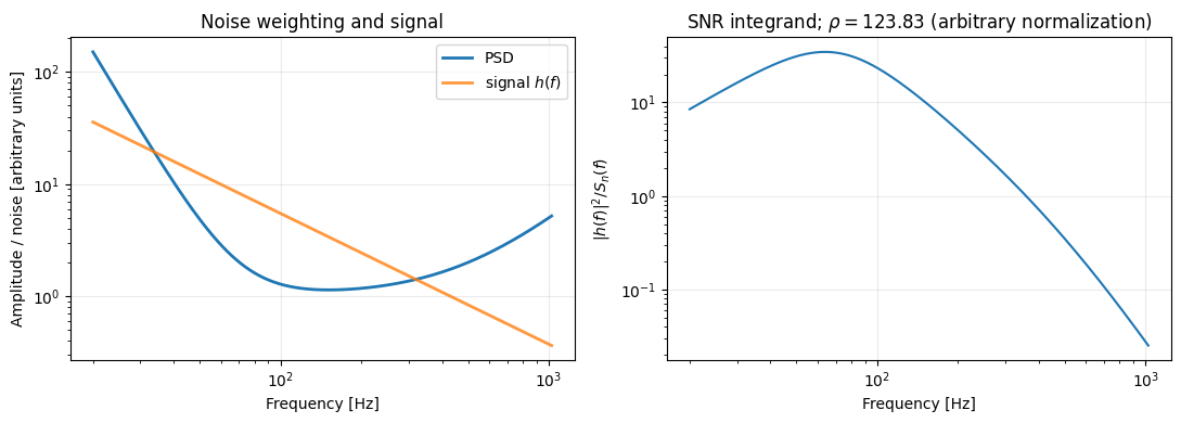
A detector’s one-sided noise power spectral density \(S_n(f)\) describes how strain-noise power is distributed over frequency (units of strain\(^2\)/Hz). Dividing by \(S_n(f)\) downweights noisy bands and gives more weight to frequencies where the detector is quieter.

Matched filtering comes from comparing the data with a candidate waveform in the presence of noise. For stationary Gaussian noise, the likelihood depends on the squared, PSD-weighted residual. This defines a noise-weighted inner product:

\[ (a|b)=4\,\mathrm{Re}\int_{f_L}^{f_H}\frac{\tilde a(f)\tilde b^*(f)}{S_n(f)}\,df. \]

The integral adds information from each frequency in the analysis band: in the discrete picture, the independent frequency-bin contributions are summed, and in the continuous limit this becomes an integral. Each bin is weighted by its noise level. Fourier transforms also make arrival-time shifts simple phase changes, so the correlation can be evaluated efficiently over many times. The real part gives a real correlation; the factor of 4 follows from using a one-sided PSD and positive frequencies only.

Here is the link from the noise model to SNR. If the signal is \(Ah\), the measured data are \(d=Ah+n\), so the residual \(d-Ah\) should look like noise. For stationary Gaussian noise, the probability of that residual is

\[p(d|A,h)\propto\exp\!\left[-\frac12(d-Ah|d-Ah)\right].\]

To ask whether the data favor a signal over noise alone, compare this likelihood with the \(A=0\) likelihood. Taking the log ratio and expanding the inner product gives

\[\ln\Lambda(A)=-\frac12\big[(d-Ah|d-Ah)-(d|d)\big]=A(d|h)-\frac{A^2}{2}(h|h).\]

The first term rewards a template that aligns with the data; the second penalizes its size. Maximizing over the unknown amplitude (allowing either sign, equivalent to a phase shift by \(\pi\)) gives \(\hat A=(d|h)/(h|h)\) and \(\ln\Lambda_{\max}=(d|h)^2/[2(h|h)]\). This motivates the signed, normalized matched-filter SNR

\[\rho_h=\frac{(d|h)}{\sqrt{(h|h)}},\qquad 2\ln\Lambda_{\max}=\rho_h^2.\]

The denominator normalizes by the template’s noise-weighted size, making the SNR unit-variance for noise alone. If the data contain the exact signal \(h\) (unit amplitude), its expected SNR is \(\sqrt{(h|h)}\), the optimal SNR. In a network of independent detectors, SNRs combine in quadrature: \(\rho_{\rm net}=\sqrt{\sum_I\rho_I^2}\).

# A toy PSD: broad low-frequency noise plus a high-frequency rise.
frequency = np.linspace(20, 1024, 2000)
mc_bns = chirp_mass(1.4, 1.4)
mc_heavier = chirp_mass(10.0, 1.4)

def inspiral_shape(f, mc):
    return 1000*mc ** (5 / 6) * f ** (-7 / 6)

psd = 1.0 + (70 / frequency) ** 4 + (frequency / 500) ** 2
h = inspiral_shape(frequency, mc_bns)
integrand = h**2 / psd
rho_squared = 4 * np.trapz(integrand, frequency)
rho = np.sqrt(rho_squared)

fig, axes = plt.subplots(1, 2, figsize=(11, 4))
axes[0].loglog(frequency, psd, label="PSD", linewidth=2)
axes[0].loglog(frequency, h, label=r"signal $h(f)$", linewidth=2, alpha=0.8)
axes[0].set(
    xlabel="Frequency [Hz]",
    ylabel="Amplitude / noise [arbitrary units]",
    title="Noise weighting and signal",
)
axes[0].legend()
axes[0].grid(alpha=0.25)

axes[1].loglog(frequency, integrand)
axes[1].set(
    xlabel="Frequency [Hz]",
    ylabel=r"$|h(f)|^2/S_n(f)$",
    title=rf"SNR integrand; $\rho={rho:.2f}$ (arbitrary normalization)",
)
axes[1].grid(alpha=0.25)

plt.tight_layout()
plt.show()

../_images/69283c3726d7f047fc1228af47bd42f4eba2f6b2fd862f75e0432786db788988.png

1.3 Template banks, matched filtering, and false-alarm rates#

Start with the template bank#

A compact-binary search does not know the signal’s component masses, spins, coalescence phase, or exact arrival time in advance. It builds a template bank: a discrete collection of modeled waveforms spanning the parameter space. The bank is designed so that the true signal is sufficiently similar to at least one template; the fractional loss in recovered signal-to-noise ratio from using the nearest template is called the mismatch. A denser bank usually reduces mismatch but increases computation and the number of noise opportunities to generate loud triggers.

Note: exaplain difference between a full PE and a low-latency search.

Matched-filter computation#

For a template \(h\) and strain data \(d\), first weight each Fourier-frequency bin by the detector noise PSD. With the one-sided PSD convention used above, define

\[ (a|b)=4\,\mathrm{Re}\int_{f_L}^{f_H}\frac{\tilde a(f)\tilde b^*(f)}{S_n(f)}\,df,\qquad \sigma_h^2=(h|h). \]

At one trial coalescence time and phase, the normalized matched-filter output is \(\rho_h=(d|h)/\sigma_h\). In a real search, the filter is evaluated over many time shifts, and phase is usually maximized over using two orthogonal phase templates (equivalently the magnitude of a complex filter output). The search repeats this calculation across templates and detectors, then clusters nearby triggers so one signal/noise excursion is not counted many times. In ideal stationary Gaussian noise, a normalized filter output has a predictable noise distribution; real detector data also contain non-Gaussian glitches and non-stationarity.

The optimal SNR is different: it is the expected signal strength if the waveform and parameters are exactly known, \(\rho_{\rm opt}=\sqrt{(h|h)}\). It has no random noise realization in it. A matched-filter SNR is an observed statistic in data, with noise fluctuations and possible template mismatch.

From search background to FAR#

A search estimates how often noise alone produces triggers at least as loud as a candidate. It constructs a background from data not containing the astrophysical on-source coincidence—for example, by shifting detector trigger times relative to each other so genuine coincident signals no longer line up, or by using off-source data. The complete search statistic is applied to that background, and the loudest background events are counted. If \(N_{\rm bg}(\geq x)\) background events have ranking statistic at least \(x\) in background live time \(T_{\rm bg}\), then

\[\mathrm{FAR}(\geq x)=\frac{N_{\rm bg}(\geq x)}{T_{\rm bg}}. \]

Search pipelines account for their bank, event clustering, detector coincidences and ranking-statistic construction when building that background.

SNR and significance are related but not interchangeable. A larger matched-filter SNR is generally more signal-like, but a raw SNR does not specify the FAR: loud glitches can have high SNR, and the background depends on the search, detector state, template bank, observing time, and ranking statistic. Searches often reweight SNR using signal-consistency tests (such as a chi-squared test) and then compare that ranking statistic with the empirical background. Therefore \(\rho>9\) alone is neither a universal detection threshold nor a FAR/significance statement.

The repository’s optimal-to-matched-filter-like SNR conversion#

The paper defines its detectability range using an SNR threshold. In the public gw_tdr implementation, the user can choose either optimal SNR (opt) or a stochastic matched-filter-like proxy (mf). The mf conversion implemented in aux_snr_mf.py is

\[k\sim\mathrm{Uniform}(0.9,1.0),\qquad X\sim\chi'^2_{\nu}\!\left(\Lambda\right),\qquad \nu=2N_{\rm IFO},\quad \Lambda=(k\rho_{\rm opt,net})^2,\qquad \rho_{\rm MF,like}=\sqrt{X}.\]

Here \(N_{\rm IFO}\) is the number of included interferometers, \(\nu\) is the chi-squared degrees of freedom, and \(\Lambda\) is its noncentrality parameter. The noncentral chi-squared draw represents the squared magnitude of \(N_{\rm IFO}\) complex matched-filter outputs: each detector contributes two phase quadratures, with the signal power set by the scaled optimal network SNR. The factor \(k\) is independently sampled between 0.9 and 1.0 to allow a modest reduction from the ideal optimal SNR. The output is stochastic, and the noise quadratures mean \(\rho_{\rm MF,like}\) is not simply \(k\rho_{\rm opt,net}\).

Important distinction: this is the repository’s approximate conversion for its mf option, not a substitute for filtering real detector data, applying a search’s signal-consistency reweighting, or measuring its FAR. The opt option uses \(\rho_{\rm opt,net}\) directly; the mf option uses the random proxy above. In either case, the TDR is conditional on the selected SNR cut and does not itself calculate a search FAR. Record the SNR convention and threshold with every result.

1.4 Paper schematic: targeted detectability range#

Ronchini et al. (2026) condition GW detectability on information from an external messenger.

Inputs — trigger time; operating detectors and their noise PSDs; waveform/mass choices; source sky localization; inclination prior; SNR threshold.

Calculation

Estimate each detector PSD from 256 s of strain (Welch: 16 s segments, 50% overlap).
Generate reference SNR samples: TaylorF2 for BNS, IMRPhenomNSBH for NSBH; integrate over 30–1024 Hz.
Draw sky positions from the messenger sky map (or hold a precise position fixed) and draw isotropic inclinations, e.g. \(0\)–\(45^\circ\) or \(0\)–\(90^\circ\).
Rescale SNR by distance and antenna/effective-distance response; combine online-detector SNRs in quadrature.
Find the distance where the required fraction of draws remains above threshold:

\[P(\rho_{\rm net}>\rho_{\rm cut})=\lambda,\qquad \mathrm{TDR}=D_{90}\ (\lambda=0.9).\]

Interpretation — \(D_{90}\) is the distance at which 90% of the assumed, prior-conditioned source draws exceed the chosen SNR cut. Since SNR scales as \(1/D_L\), it is the 10th percentile of the draws’ threshold horizons.

Caveat — This is a source-informed detectability estimate, not a search FAR or exclusion distance. The paper compares TDR with targeted-search 90% exclusion distances and finds a population-level correlation; the two quantities are not identical.